Fabric Law for Elastic Orthotropic Shells (LAW19 and LAW58)

Two elastic linear models and a nonlinear model exist in Radioss.

Fabric Linear Law for Elastic Orthotropic Shells (LAW19)

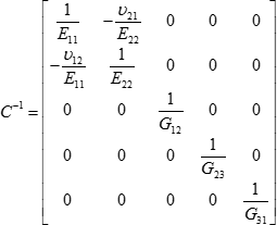
A material is orthotropic if its behavior is symmetrical with respect to two orthogonal plans. The fabric law enables to model this kind of behavior. This law is only available for shell elements and can be used to model an airbag fabric. Many of the concepts for this law are the same as for LAW14 which is appropriate for composite solids. If axes 1 and 2 represent the orthotropy directions, the constitutive matrix

C

is defined in terms of material properties:(1)

where the subscripts denote the orthotropy axes. As the matrix

C

is symmetric:(2)

\frac{υ_{12}}{E_{11}} = \frac{υ_{21}}{E_{22}}

Therefore, six independent material properties are the input of the material:

$E_{11}$: Young's modulus in direction 1
$E_{22}$: Young's modulus in direction 2
$υ$ ₁₂: Poisson's ratio
$G_{12}$ , $G_{23}$ , $G_{31}$: Shear moduli for each direction

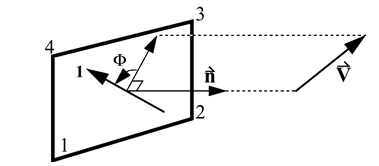
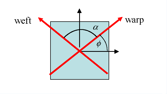
The coordinates of a global vector $\vec{V}$ is used to define direction 1 of the local coordinate system of orthotropy.

The angle

Φ

is the angle between the local direction 1 (fiber direction) and the projection of the global vector

\vec{V}

as shown in Figure 1.

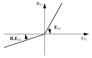
The shell normal defines the positive direction for

Φ

. Since fabrics have different compression and tension behavior, an elastic modulus reduction factor, R_E, is defined that changes the elastic properties of compression. The formulation for the fabric law has a

σ_{11}

reduction if

σ_{11}

< 0 as shown in Figure 2.

Fabric Nonlinear Law for Elastic Anisotropic Shells (LAW58)

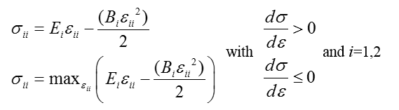
This law is used with Radioss standard shell elements and anisotropic layered property (TYPE16). The fiber directions (warp and weft) define the local axes of anisotropy. Material characteristics are determined independently in these axes. Fibers are nonlinear elastic and follow the equation:(3)

The shear in fabric material is only supposed to be function of the angle between current fiber directions (axes of anisotropy):(4)

\begin{array}{l} τ = G_{0} \tan (α) - τ_{0} if α \leq α_{T} \\ τ = G \tan (α) + G_{A} - τ_{0} if α > α_{T} \end{array}

and

$G_{A} = (G_{0} - G) \tan (α_{T})$ , $G = \frac{G_{T}}{1 + \tan^{2} (α_{T})}$ with $τ_{0} = G_{0} \tan (α_{0})$

Where,

α_{T}

is a shear lock angle,

G_{T}

is a tangent shear modulus at

α_{T}

, and

G_{0}

is a shear modulus at

α

= 0. If

G_{0}

= 0, the default value is calculated to avoid shear modulus discontinuity at

α_{T}

G_{0}

G

$α_{0}$ is an initial angle between fibers defined in the shell property (TYPE16).

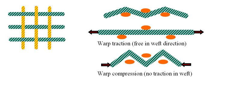
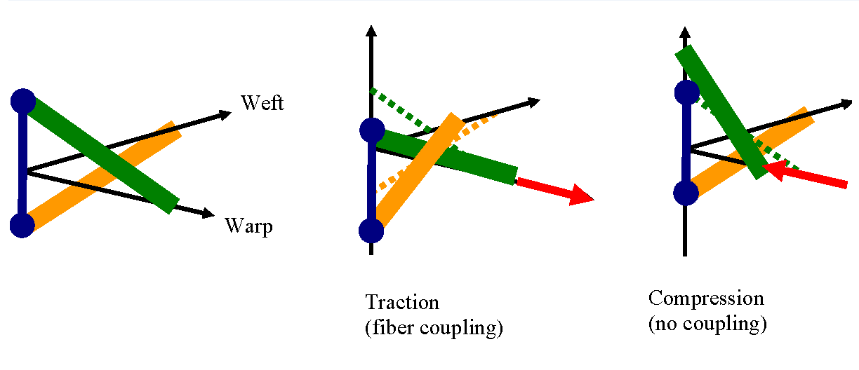
The warp and weft fiber are coupled in tension and uncoupled in compression. But there is no discontinuity between tension and compression. In compression only fiber bending generates global stresses. Figure 4 illustrates the mechanical behavior of the structure.

A local micro model describes the material behavior (Figure 5). This model represents just ¼ of a warp fiber wave length and ¼ of the weft one. Each fiber is described as a nonlinear beam and the two fibers are connected with a contacting spring. These local nonlinear equations are solved with Newton iterations at membrane integration point.