acm (general)
Consolidates several ACM definitions into one general, flexible ACM definition. Besides mid thickness, constant thickness, and maintain gaps, the definition of several coats with different hexa patterns is available.
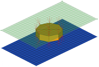
Figure 1.
ACM Realization Options
| Option | Action |
|---|---|
| thickness | Select a thickness
option used for dimensioning and positioning hexas.
|
| num hexas | Create a hexa cluster
with 1, 4, 8, 12, 16 or 32 hexas, which are arranged in a
predefined pattern.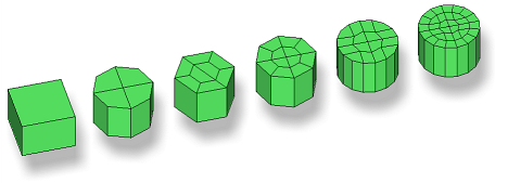 Figure 4. Note: Available for all ACM realization
types.
|
| coats | Define the number of hexa elements required along the thickness. Multiple solid coats are supported. |
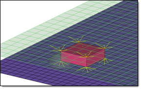
| orthogonal faces | Force the creation of
perfectly orthogonally-shaped hexas.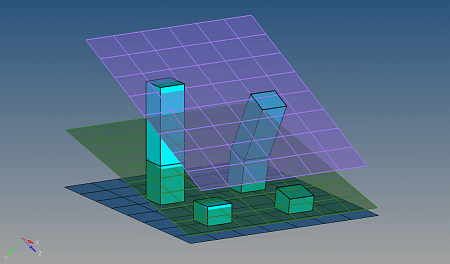 Figure 5. . The two leftmost realizations were performed with the orthogonal faces option enabled. Note: Available for any kind of ACM weld, if num hexas is
set to 1.
|
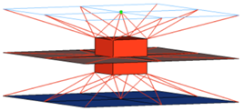
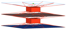
| use rbe3 radius | RBE3 elements are
typically created with three or four legs dependent on the
element type (quadface, triaface) the projection of the
appropriate hexa node is landing on. To be more accurate,
especially regarding different mesh sizes, an rbe3 radius can be
defined, so that more nodes nodes can be joined by each RBE3
element. In any case, at least one element face will be joined
by each RBE3 element.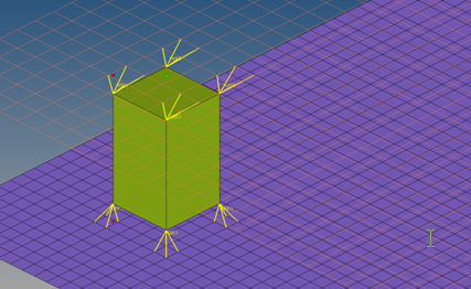 Figure 6. use rbe3 radius Disabled 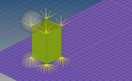 Figure 7. use rbe3 radius Enabled All of the nodes of the appropriate link (outer nodes, if it is a solid link), which are positioned inside a sphere around the projection point, are considered to be joined to the RBE3 element. A feature angle is also considered. The nodes that are on a different side of the feature edge than the projection point will not be joined to the RBE3 element. When enabled you must define:
Note: Only available for the realization type acm
(general).
|