Slope
Captures the slope of the curve derived from two expressions at a particular instance of time.
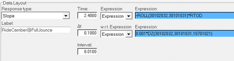
Figure 1. Response Type – Slope
| Input | Description |
|---|---|
| Expression |
|
| w.r.t. Expression |
|
| Time | The simulation time at which the slope of curve (which is derived using Expression as ordinate and w.r.t. Expression as abscissa) is desired. |
| ∆t | Typically a small time value that is used to pick two points (one at Time+∆t and other at Time-∆t) on the derived curve for calculating its slope. |
| Interval | A ‘Time Tolerance’ value used by four ‘At Time’ responses (in other words, two responses for Expression and two for w.r.t. Expression) that are generated internally to obtain the two points on a derived curve. |
In the above example, the response variable computes the slope of curve with Roll position (Ride Camber) plotted on its Y axis and marker’s relative displacement in Z (Full Jounce) plotted on its X axis at a time value of 2.4.