Spline2D/Curves

Use the Spline2D/Curves tool to create and edit curves.

Curves Overview

A curve consists of two or more column vectors that can be used either to create XY data (referred as 2D spline) or a line geometry in 3D modeling space (3D curve). The 2D spline can be used as reference input for other MotionView entities such as a force or motion. The 3D curve can be used for certain types of constraints such as a Point to Curve (PTCV) constraint.
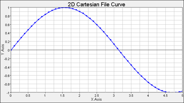


Figure 1.

Curves have many varies applications, some of which are listed below:

Application Description
Forces Forces are used to define nonlinear characteristics for the forces. The curve may represent a spring force versus deformation characteristic or a damping force versus deformation velocity characteristic. This data is frequently measured experimentally.
Motions Motions are used to define nonlinear displacements versus time, velocity versus time, and/or acceleration versus time
Vectors, Differential equations Curves may be used to define relationships that are difficult to describe analytically.
Note: A 3D curve can also be used for certain types of constraints, such as a Point-to-Curve constraint.
There are two types of curves that can be defined in MotionView:
  • 2D Curves
  • 3D curves
Each of the above types can further be defined as a:

Cartesian Curve

A Cartesian curve simply consists of two or more vectors that could be defined independent to each other, yet they should consist of same number of data points.

Paramteric Curve

A Parametric curve is defined in terms of one free parameter, u. Referring to the image below, assume a curve C is defined with respect to a coordinate system OXYZ. The coordinates of any arbitrary point on the curve P, as measured in OXYZ, can be represented uniquely in terms of the free parameter u with three functions, f(u), g(u), and h(u), that define the x-, y- and z-coordinates of P. The extent of the curve is governed by the start and end values of u. This is a parametric representation for a curve.
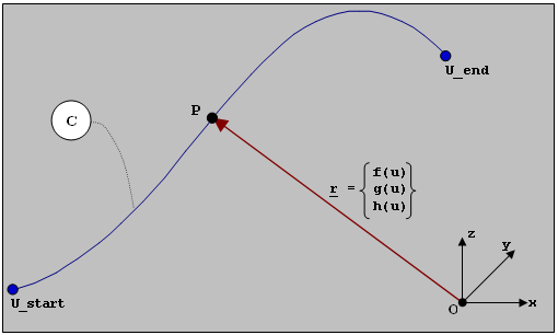


Figure 2.

A 2D Parametric curve has three vectors – that is, one free parameter vector U, and two dependent vectors X and Y.

A 3D parametric curve has fours vectors – that is, one free parameter U, and three dependent vectors X, Y, and Z.

Create Curves

The Curves tool to create and edit curves.

  1. From the Project Browser, select the system to which the curve is to be added.
  2. Right-click on a system in the Project Browser and select Add > Reference Entity > Curve from the context menu.
    OR
    Right-click on a curve folder in the Project Browser and select Add Curve from the context menu.
    OR
    From the Model ribbon, Splines tool set, click the Spline2Ds(Curves) icon.
    The Add Curve dialog is displayed.
  3. Specify a label for the curve.
    The curve label can be changed at any time.
  4. Specify a variable name for the curve.
    By default, variables names of entities in MotionView follow a certain convention. For example, all curve entities have a variable name starting with “crv_”. This is the recommended convention to follow when building models in MotionView since it has many advantages in model editing and model manipulation.
  5. Click OK to close the window or Apply to continue creating entities.
    Once a curve entity has been added to the model, the panel for the curve will automatically be displayed in the panel area.

Edit Curves

In MotionView, a curve entity is used to capture non-linear characteristics of forces and motion or to describe constraint paths for high-pair joint types. A 2D curve is used to represent the non-linear characteristics of forces or motion and a 3D curve can be created to use in a higher pair joint.

Define the Properties of Curves

From the Properties tab, you can define and edit the curve properties listed below.

  1. If the Curves panel is not currently displayed, select the desired curve by clicking on it in the Project Browser or in the modeling window.
    The Curves panel is automatically displayed.
  2. From the first drop-down menu, select whether to define a 2D/3D Cartesian curve or a 2D/3D parametric curve.
  3. Select the u, x, y, or z radio buttons (depending on your selection in the previous step) and choose File, Math or Values as the data source for the curve from the corresponding drop-down menu.
  4. Define the data source.
    If File is chosen:
    1. Click the file browser to select the data files for the x and y vectors.
    2. Define the Type, Request, and Component options for each vector.
      Depending on the file chosen, the options may already be filled in.

      MotionView supports several commonly used file formats such as .csv and .txt, as well as other data formats supported by HyperGraph such as .abf, .plt, .dac, .rsp, and so on.

      The curve reader can handle multiple blocks of data in the file and arrange them into Type, Requests and Components. The Type and Requests are blocks and sub-blocks of data and a component is a vector (or column) within the sub-block.

      While using a .csv or a .txt as a data file, set the Type to Unknown. Request will appear as Block 1. If headers are specified for columns, those headers will appear under Component. Otherwise, they would be listed as Column 1, Column 2, and so on.


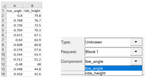
      Figure 3. CSV file columns when read as a curve in MotionView
    3. Enter a value in the Start Index field to specify the index number of the first data point in the subrange.
      The default is 1.
    4. Enter a value in the End Index field to specify the index number of the last data point in the subrange.
      The word "last" can be used to specify the last data value in the file without knowing how many data points are in the file.
    5. Enter a value in the Increment field to specify the number of points to advance when reading the subrange.
      For example, to read every data point in the file, enter an increment value of 1; to read every other data point, enter a value of 2. The default is 1.
      Tip:
      • Click Reload data to reload the contents from the selected file into memory.
      • Click View File to display a Preview dialog that contains the text version of the file.
    If Math is chosen, the curve calculator is displayed, allowing you to define the vector mathematically. Below are two sample expressions:
    Expression Description
    crv_2d_math.x = 0:10:1 X vector expression to generate a series of numbers from 0 to 5 at regular intervals of 0.1.
    crv_2d_math.y = cos(crv_2d_math.x) Y vector expression to apply a cosine function on the X vector of the curve.
    If Values is chosen, enter the u, x, y, and z data values for each point. You can cut, copy, paste and insert data point values using the buttons to the right of the table.
    Note: The available data points will depend on your curve type selection in the first-drop-down menu.
    Tip: Click to view the Data Values dialog containing all data points.

    For more information on the Type, Request, and Component options, see Building Plots with XY Data Files in the HyperGraph on-line help.

  5. From the second drop-down menu, specify if the curve will be written to the solver file.
    This option determines if the curve data is exported to the solver input deck.
  6. From the third drop-down menu, select Curve points or Control points.
    This option determines if the points are to be exactly on the curve (curve points) or used to fit the curve (control points).
  7. From the fourth drop-down menu, select Open Curve or Closed curve.
    This options determines whether or not the first and last point should be connected for a closed curve. Choosing Closed curve results in a continuous path for a constraint using this curve.
Tip:
  • Click Show Curve to display a curve preview dialog.
  • Click Export Curve to display the Export Curve dialog, which allows you yo export plot data in several different formats that can be read by other software applications. See the Export a Curve topic for additional information.

Define the Attributes of Curves

From the Attribute tab, you can define the scale and offset for the X and Y vectors. When a data vector is scaled, the vector is multiplied by a specified value. The original data values are not actually altered. Offsetting a data vector shifts the data along the corresponding axis.

  1. Click the Attributes tab.
  2. Enter values in the Scale and Offset fields for the U, X, Y, and/or Z directions (depending on your selections in the Properties tab).
    You can also enter math expressions, such as one for converting Fahrenheit to Celsius, in the scale and offset fields.
Tip: Checking the Linear Extrapolation box results in the lin_extrap flag being used by the solver. Linear extrapolation enables the solver to extrapolate the curve linearly when the computed value for the independent variable goes out of the specified bounds.

Define the Visualization of Curves

From the Visualization tab, you can define the way you want to display, or visualize, a curve.

Note: This tab only becomes available for 2D cartesian curves of the type File and Math.
  1. Click the Visualization tab.
  2. Activate the Extrapolate option and enter the percentage by which you want to extrapolate the curve.
  3. Activate the Interpolate option.
  4. From the drop-down menu, select a method to interpolate the curve:
Tip:
  • Click Show Curve to display the curve Preview dialog.
  • Activate Symbols to place symbols on a curve to indicate data points.

User-Defined Properties for a Curve

If desired, define the curve using the User-Defined tab, which will allow you to specify the properties of the curve using user subroutines.

  1. From the Properties tab, click the User-defined check box.
  2. Click the newly added User-Defined tab.
  3. Define the user subroutine.
    1. Provide an expression with the USER solver function with parameters being passed to the user subroutine.
    2. Alternatively, activate the Use local file and function name check box to specify a local file where the subroutine code can be accessed by the solver.
      If this option is not specified, MotionSolve will search for a subroutine following its user subroutine loading rules.
    3. Select a function type from the drop-down menu.
    4. Select the local file for the subroutine.
      The type of file to be specified will depend on the selected function type. For example, if DLL/SO is selected, you can specify a file with a .dll extension (for Windows) or an .so extension (for Linux).
    5. Specify the function name in the subroutine that defines the entity, or accept the default name provided by HyperWorks.

Export a Curve

Plot data can be exported in several different formats that can be read by other software applications.

  1. From the Properties tab, click the Export Curve button to display the Export Curve dialog.
  2. Select a format for the exported data from the Type drop-down menu.
    Export types for the following ASCII file types are included:
    Type File Path Description
    Excel .csv CSV, comma separated values format. CSV is compatible with most spreadsheet applications. Commas delimit the data.
    Columns .col One column for X data and another for Y data. A blank line separates each curve in the plot. Tabs delimit the data.
    XY Data .dat One column for X data and another for Y data. The data set for each curve in the plot begins with XYDATA and ends with ENDATA. The XY units and the axis labels are included at the top of each data set. Tabs delimit the data. HyperMesh uses this format.
    X Graph .xrg One column for X data and another for Y data. The XY units and the axis labels are included as comments at the top of each data set. Tabs delimit the data.
    Summary .sum The summary file contains the plot title and a table listing the curves in the plot, the X and Y data labels, and the min and max values of each curve.
    ADAMS Spline .adm The X values for each curve are listed in comma delimited columns followed by the Y values in comma delimited columns. The first data set in the file is labeled SPLINE/0. The label for each successive data set is incremented by one.
    Altair Binary .abf All curves in the window are written to an Altair Binary format file.
    DAC .dac Exports curve data to DAC files, one file per curve. If more than one curve is requested, the name of the output file is modified by adding the unique request name to the file name.
    RPC .rsp Exports curve data to RPC files, with all curves going to one file.
    Excel Europe .csv Writes out a file with the CSV extension, but uses a semi-colon instead of a comma to separate columns.
    User-specified formats .

    User-specified import templates and external readers can be created.

    See the HyperGraph online help for additional information.

    Note: Export templates can be added to the Export Curve dialog using the *AddExportFormat() statement in the preference.mvw file.

    See MotionScript Reference for more information on adding export formats.

    Export format templates are written using the Templex programming language.

  3. In the File field, enter a name for the exported file.
    The file is stored in the selected directory using the file browser or the directory from which the program was started. The default file name is export.ext, where ext indicates the file type specified in the export template.