Tutorial: Explore Three Coupling Methods with Flux
Compare three coupling methods between Activate and Flux using co-simulation, lookup
tables and FMUs.
Co-Simulation Method
This is a dynamic approach in which Flux and Activate run simultaneously to
produce very accurate results at the cost of a longer run time. The
co-simulation is initiated from Activate between the Activate model
Actuator_Coupling.scm and the 2D
transient magnetic Flux model MultiPhysics.FLU. The co-simulation is dependent on the kinematics that is
defined in Flux 2D through the analysis option, multi-physics position. The
Flux model provides values to the Activate model including force, current and
speed through the Flux block in the coupling component. In Activate, the Flux
block is defined to receive values for position and voltage as input.
Lookup Table Method
This approach includes two separate simulations: The first includes opening the
FEA model Static_no_solved.FLU in Flux and
running an analysis in magneto-static mode. Simulation results for Current,
Position and Flux are produced as .oml script files. A second simulation is
performed in Activate where the Flux results are read in from the .oml script
files by way of a Lookup Table ND in the Activate model.
FMU Method
This approach includes two separate simulations: The first includes opening the
FEA model Static_no_solved.FLU in Flux and
running an analysis in magneto-static mode. Simulation results for Current,
Position and Flux are exported as Functional Mock-up Unit files. A second
simulation is performed in Activate where the Flux results are imported from the
.fmu files by way of an FMU Import block.
Files for This Tutorial
Primary files include: MultiPhysics.FLU (the Flux
contactor model file), Actuator_Coupling.scm (the Activate model
file) and Static_no_solved.FLU (the Flux
lookupND table)
A finished version of the models you build in the
tutorials along with any files required to complete the tutorials are available at this
location:
<installation_directory>/tutorial_models/Flux_Actuator_Variants
and are accessible from the Demo Browser.
ImportantColonSymbol The co-simulation
process requires that the FLUX .FLU and
.F2STA files be located in the same working directory. When
naming the working directory, avoid spaces and special characters as Flux cannot
recognize them.
Overview of the Flux Projects
The Flux projects with all of the required files for each of the simulation methods
discussed in this tutorial are available from the Demo Browser:
/tutorial_models/Flux_Actuator/.
Flux Applications
Magneto Static
Transient Magnetic
Flux Main Functions
Translation motion, Mechanical set (For more details, see Flux
Supervisor examples in the Flux help)
Kin. = multi-static application and multi-physics position
Generate OML
Generate Activate coupled component
Generate FMU
Flux Post-Processed Quantities
Magnetic quantities
Kinematic quantities
Circuit quantities
2D curve analysis
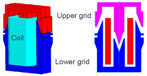
Flux Contactor (Trident) Model
The main Flux contactor model MultiPhysics.FLU is comprised of
three main components:
A lower grip, ferromagnetic fixed part
An upper grip, ferromagnetic (laminated) moving part assembled on
springs
A coil placed around the central tooth
Python Files for Flux Projects
The Flux project folders contain the completed Flux results for all three
simulation methods. If you want to experiment with launching the simulations on
your own or if you want to use your own coupling file, the Python files for you
to do so are available in the Flux projects for all three simulation methods:
Co-simulation = Coupling_Component.py
OML = Generate_OML.py
FMU = Generate_fmu.py
Overview of the Activate Model Files
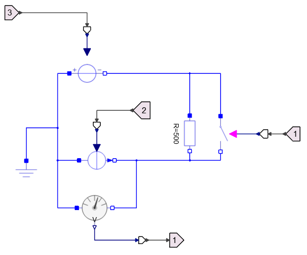
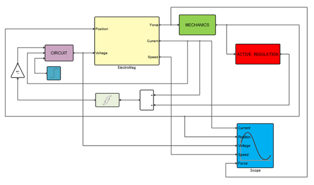
Activate Coupling Model
Figure 1. Actuator_Coupling.scm
Electric Circuit
The purple CIRCUIT super block in the coupling model is comprised of four main
components:
a controlled switch that opens and closes based on voltage
a resistor that serves to prevent short circuiting
a current and voltage input
a voltage output sensor
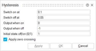
Regulation Command
A simple regulation command in the coupling model is included in the light
green Hysteresis block. Here the model is dependent on the active regulation
of time.
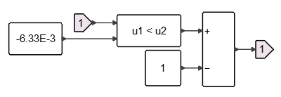
Active Regulation
In the red ACTIVE REGULATION super block, we compare two values and use this to
activate the Hysteresis regulation.
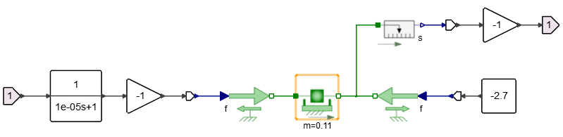
Mechanical Equation
The bright green super block, MECHANICS, includes Modelica blocks to simulate
the mechanical part of the device and position the actuator.
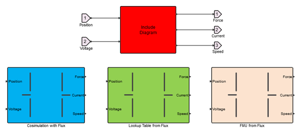
ElectroMag Super Block
The ElectroMag super block (yellow) of the Activate Coupling model (Actuator_Coupling.scm) contains the electromagnetic component of
the model and consists of the Include Diagram block (red) and three
additional super blocks: Cosimulation with Flux
(blue), Lookup TableND from Flux (green) and
FMU from Flux (pink) that you see in the
following diagram. The Include Diagram block defines which super block to
call into play depending on which simulation method you specify through the
Mode variable. The super blocks are inactive otherwise.
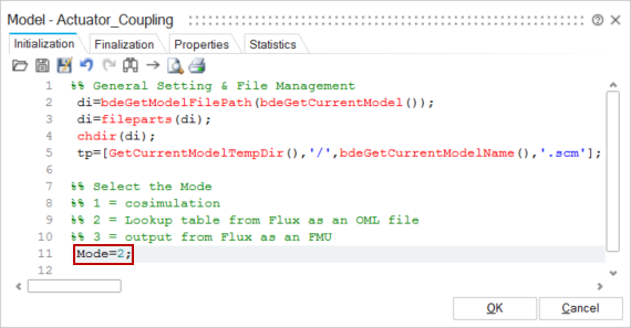
Model Variants
The Activate model
Actuator_Coupling.scm is configured to
implement three methods of simulating the Flux contactor with and Activate actuator in
one model. In practice, to drive the three variants, one variable is defined in the
Initialization phase for the model. This variable is named Mode and
can be set to 1, 2 or 3.
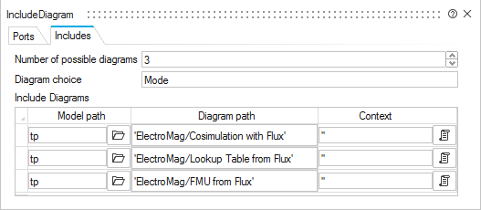
The Mode variable is used in the IncludeDiagram block to
determine which of the three super blocks to include in the simulation.Inclde Diagram block set defined for Mode 2
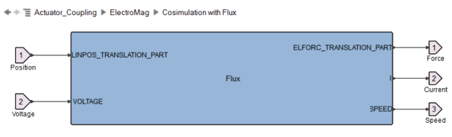
Co-Simulation Method
In Activate, open the model Actuator_Coupling.scm.
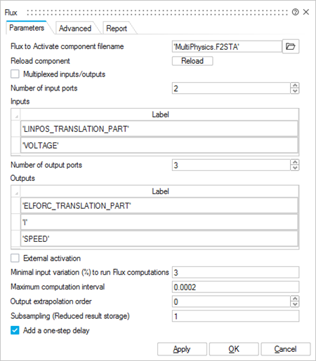
In the super block Cosimulation with Flux, the Flux
block performs the co-simulation by reading in the coupling component that
was generated using the Flux 2D transient application file
MultiPhysics.F2STA.
Look-Up Table Method
In Activate, open the model Actuator_Coupling.scm.
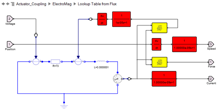
The super block Actuator_Coupling#menucascade-separatorElectroMag#menucascade-separatorLookup Table from Flux includes a context to read in the results exported from a
magnetostatics simulation in Flux.
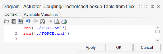
The Flux results are exported as two .oml files FLUX.oml
and FORCE.oml. These files are available in the Flux
project folder and are directly read in from the Activate model. In the
following image, the super block Lookup Table from
Flux includes the yellow blocks
LookupTableND and
LookupTableND_1 which load
FLUX.oml and FORCE.oml
respectively.
The context of this diagram includes the directions for the
FLUX.oml and FORCE.oml files
to be read into the super block.
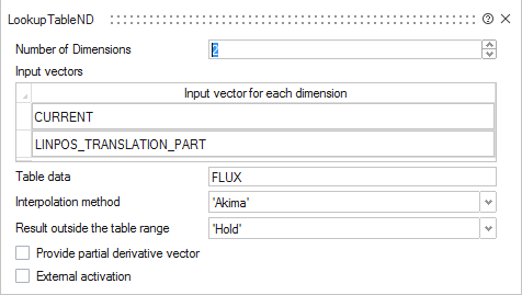
In the Lookup TableND dialog, the field Table data
calls the OML variable FLUX from the
FLUX.oml file as an interpolated function of the
two vectors CURRENT and LINPOS_TRANSLATION_PART.
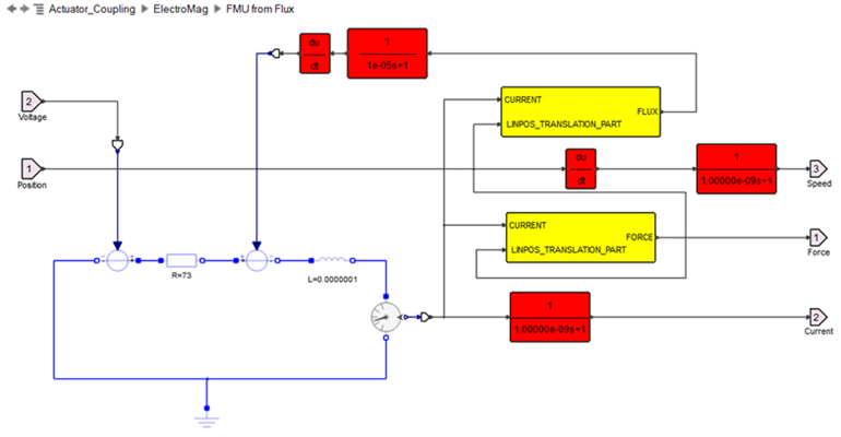
FMU Method
In Activate, open the model Actuator_Coupling.scm.
The super block Actuator_Coupling#menucascade-separatorElectroMag#menucascade-separatorFMU from Flux includes a context to read in the results exported from a
Flux 2D magnetostatics simulation.
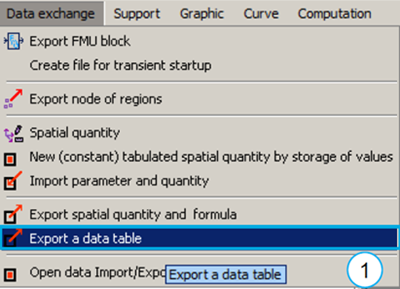
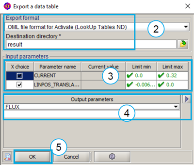
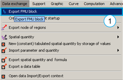
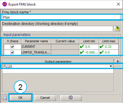
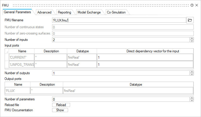
The Flux results are exported as two .fmu files:
FLUX.fmu and FORCE.fmu. The
steps in Flux to export the .fmu files are indicated in the following
dialogs:
The .fmu files are available in the Flux project folder and are directly read
in from the Activate model. In the super block FMU from
Flux, the yellow blocks are FMU and
FMU_1 that load FLUX.oml and
FORCE.oml respectively.
The Functional Mockup Interface standard is an important gateway to other
products. In this tutorial, the use of either a Lookup Table or an FMU are
almost identical and are meant to illustrate various features of Flux and
Activate.
Simulation Results
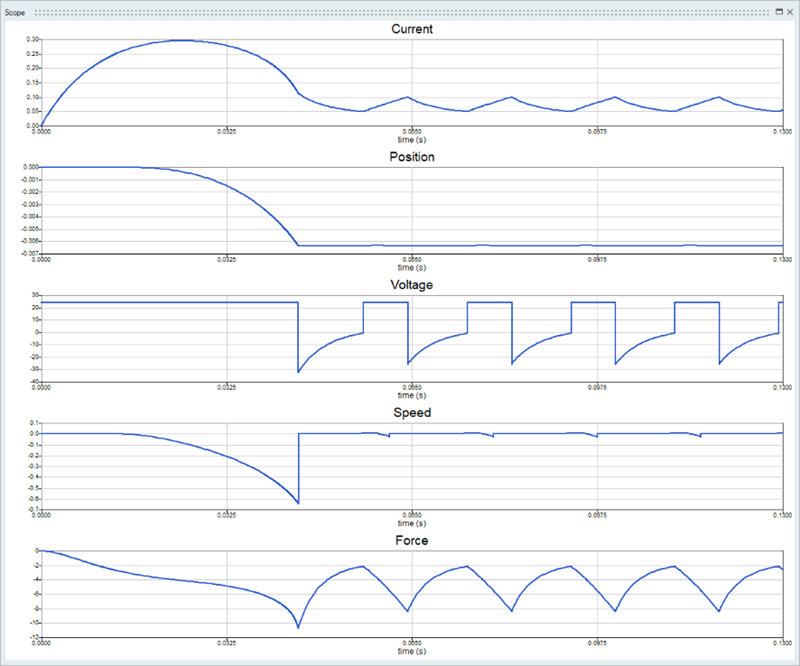
Mode 1: Co-Simulation Method
With the
co-simulation method, a Flux transient (dynamic) analysis is run directly from Activate
through the coupling component from Flux. This type of simulation is slow but can
account for Eddy current effects in massive iron conductors. The added value of the
Flux-Activate co-simulation coupling is the accuracy of the results with the inclusion
of the Eddy currents. In this case, the type of kinematics in the mechanical rotor is
multiphysics position. Note that the value of the initial
position must be determined in order to obtain the correct results. Co-Simulation results with the evolution of current, position, speed and force
as a function of time
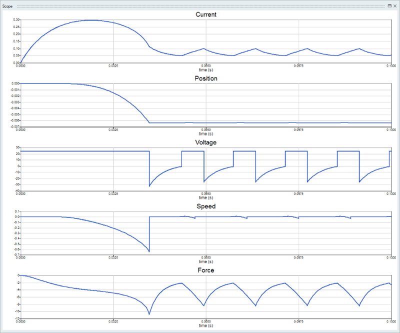
Mode 2: OML Method
The aim of this method
is to build an accurate reduced model (based on the Finite Element model) of the linear
actuator. Accuracy and quick simulation with Activate are the biggest advantages of this
approach. The linear actuator behavior is represented by the flux in the coil and the
force which are calculated with a finite element method. First, through the Flux
simulation, the response surface of flux and force is computed. In a first
approximation, the variation parameters are Current and Position. This response surface
is used in Activate. OML Method Results with the evolution of current, position, speed and force as
a function of time
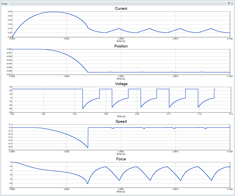
Mode 3: FMU Method
The FMU block enables
the import and simulation of an FMU as an Activate block. The FMU can be of type
Model-Exchange (ME) or Co-Simulation (CS). Both version 1.0 and 2.0 are supported.
Inputs and outputs can be of Real, Integer, Boolean or String data types. Only scalar
input and output are supported. The aim of this method is to build an accurate reduced
model (based on the Finite Element model) of the linear actuator. Accuracy and quick
simulation with Activate are the biggest advantages of this methodology. The linear
actuator behavior is represented by Flux in coil and force which are calculated with a
finite element method. In Flux, a simulation is run with a finite element method to
compute the response surface of the flux and force. In a first approximation, the
variation parameters are Current and Position. Once the simulation is finished, an FMU
file is generated. This FMU is then used in Activate. FMU Method Results with the evolution of current, position, speed and force as
a function of time
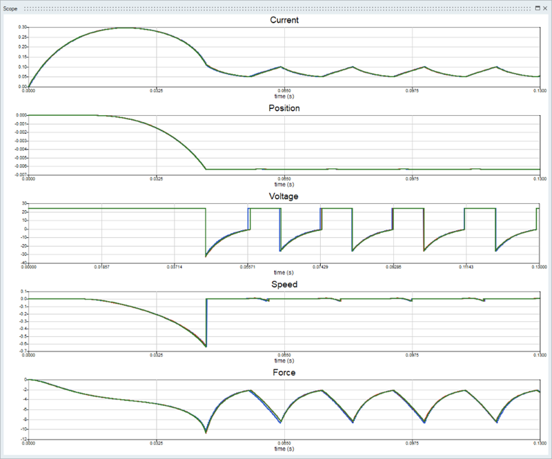
Results Comparison
Aside from the varying peaks between the three methods: co-simulation in blue, OML in
red and FMU in turquoise, the results are very similar. The small variance is due to
the different interpolation methods applied to run simulations on reduced models for
the OML and FMU methods.
Results comparison of the three simulaiton methods
 Actuator_Coupling.scm