HVVH-6000: Solution Tab
- Check run an OptiStruct or Radioss solver deck
- Compare OUT files of OptiStruct-written results files after a check run.
- Two OUT files generated from the solver run ( Radioss or OptiStruct) can be compared.
- The current solver run OUT file can be compared with the reference OUT file.
- Two OUT files generated from the same solver deck using two different solver versions can be compared.
Check Run Solver Data for a Radioss Deck
-
Click Check run.
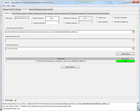
Figure 1. -
In the Input file (solver deck) field, click the file browser icon,
 , to load
the BOXBEAM_0000.rad file, located in
..\tutorials\hvvh\Solution\Radioss\Checkrun\BOXBEAM\BOXBEAM_0000.rad.
, to load
the BOXBEAM_0000.rad file, located in
..\tutorials\hvvh\Solution\Radioss\Checkrun\BOXBEAM\BOXBEAM_0000.rad.
-
In the Output directory field, click to
select an output directory.
-
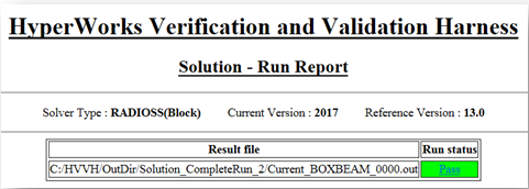
To open the HTML report, click HTML Report.
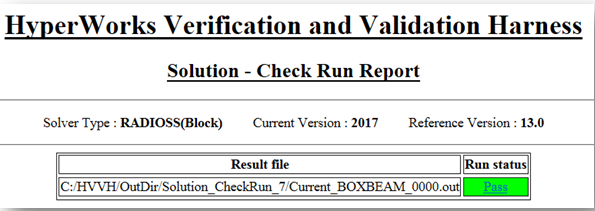
Figure 2.
Use the Out Compare Option
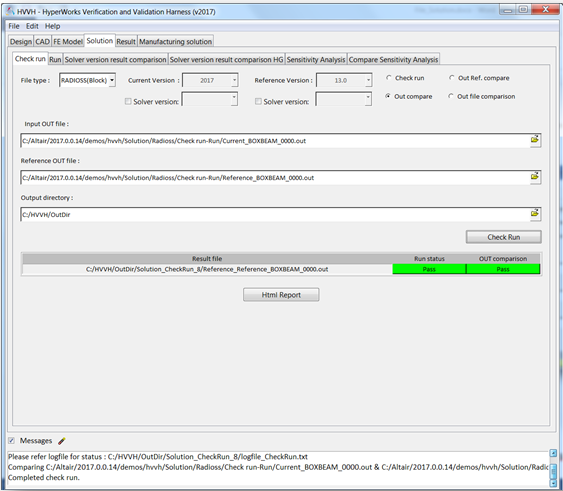
Figure 3.
-
In the Input OUT file field, click the file browser icon, , to load
the
..\tutorials\hvvh\Solution\Radioss\Checkrun\Current_BOXBEAM_0000.out
file.
-
In the Reference OUT file field, click to load
the Reference_BOXBEAM_0000.out file, locted in
..\tutorials\hvvh\Solution\Radioss\Checkrun\
file.
-
In the Output directory field, click to
select an output directory.
-
To open an HTML report, click HTML Report.
The comparison of different blocks of results are shown line-by-line. Warnings are in light orange and errors are in dark orange.
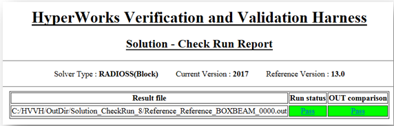 Figure 4.
Use the Out Ref. Compare Option
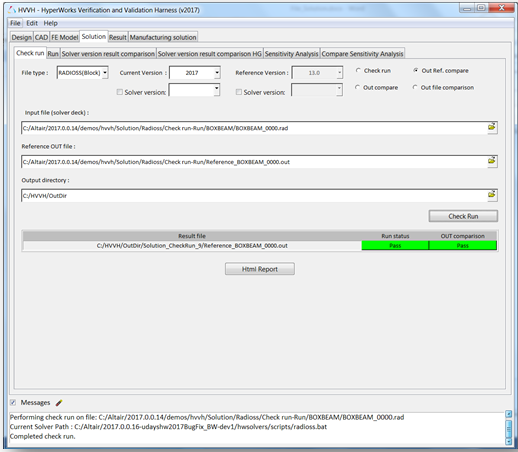
Figure 5.
-
In the Input file field, click the file browser icon, , to load
the BOXBEAM\BOXBEAM_0000.rad file, located in
..\tutorials\hvvh\Solution\Radioss\Checkrun\BOXBEAM\.
This file is used for the solver run in the background.
-
In the Reference OUT file field, click to load
the Reference_BOXBEAM_0000.out file, located in
..\tutorials\hvvh\Solution\Radioss\Checkrun\Reference_BOXBEAM_0000.out.
This file is used to compare the first generated OUT file.
-
In the Output directory field, click to
select an output directory.
-
To open an HTML report, click HTML Report .
The comparison of different blocks of results are shown line-by-line. Warnings are in light orange and errors are in dark orange.
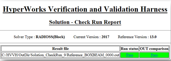
Figure 6.
Use the Out File Comparison Option
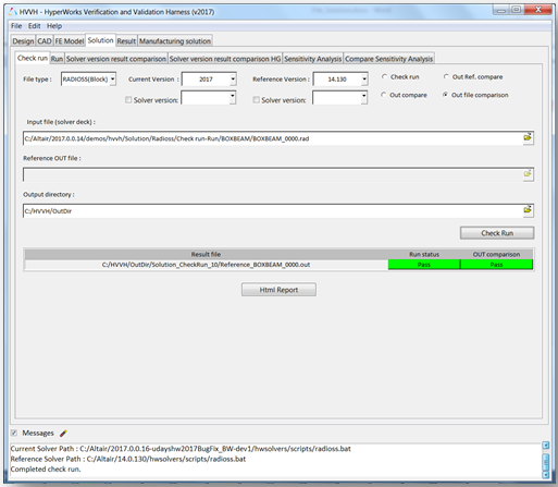
Figure 7.
-
In the Input file field, click the file browser icon, , to load
the BOXBEAM_0000.rad file, located in
..\tutorials\hvvh\Solution\Radioss\Checkrun\BOXBEAM\BOXBEAM_0000.rad.
This is the solver file that is used to run the solver for the check run. The OUT file is created in the output directory.
-
In the Output directory field, click to
select an output directory.
-
To open an HTML report, click HTML Report.
The comparison of different blocks of results are shown line-by-line. Warnings are in light orange and errors are in dark orange.
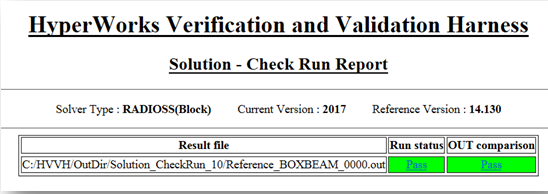
Figure 8.
Solver Run
Run the solver and compare OUT files for solver-written results files.
- Two OUT files generated from the solver run can be compared.
- The current solver run OUT file can be compared with the reference OUT file.
- Two OUT files generated from the same solver deck using two different solver versions can be compared.
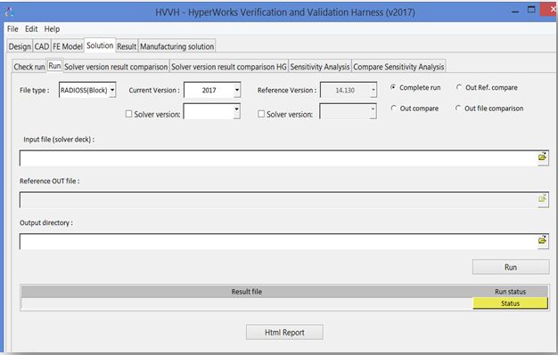
Figure 9.
-
In the Input file field, click the file browser icon, , to load
the BOXBEAM_0000.rad file, located in
..\tutorials\hvvh\Solution\Radioss\Run\BOXBEAM\.
This file is used for the solver run in the background.
-
In the Output directory field, click to
select an output directory.
-
Click HTML Report to open an HTML report.
The following three options on the Run tab work as they do on the Check run tab (see Steps Use the Out Compare Option through Use the Out File Comparison Option above).
- Out compare (out files comparison)
- Out Ref. compare (out files comparison)
- Out file comparison from solver check runs
For Radioss, both the Starter OUT file and Engine OUT files are compared.
For OptiStruct, the OUT files are compared.
Figure 10.
Solver Version Results Comparison (Radioss or OptiStruct)
-
From the Solution tab, select the Solver
version result comparison tab.
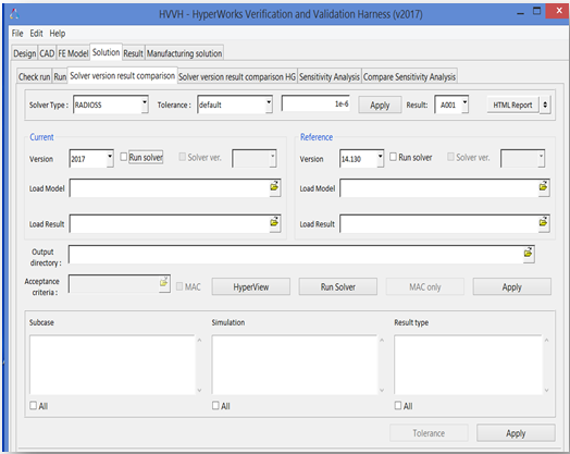 Figure 11.
 -
Under Current, in the Load Model field, click the file browser icon, ,to load
the BOXBEAM_0000.rad file file, located in
..\tutorials\hvvh\Solution\Radioss\Solver-versions-result-comparison\Current\BOXBEAM_0000.rad.
-
Under Reference, in the Load Model field, click to load
the BOXBEAM_0000.rad file, located in
..\tutorials\hvvh\Solution\Radioss\Solver-versions-result-comparison\Reference\.
-
In the Output directory field, click to
select an output directory.

Figure 12. -
Click Run Solver.
After the solver run, the A001 results are loaded in the Load Result option.
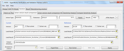
Figure 13. -
Click Apply.
The results available (Subcase, Simulation, and Result type) in the current result file are loaded in the three windows.
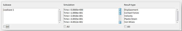
Figure 14. -
Select each All under each of the windows and click the
second Apply button.
Any combination of Subcase, Simulation, and Datatype can be selected for comparison.
Results comparison of the current and reference results are generated.
In the Messages window, the run details and the log file location are displayed.
If any difference is greater than the tolerance, it is indicated with the label Fail. Otherwise, they are labeled Pass.
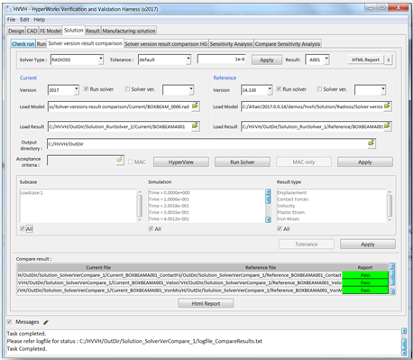
Figure 15. -
Click HTML Report to open an HTML report.
Comparisons between different data types are available.
For example, for a vector (displacement), the components magnitude, X-displacement, Y-displacement, and Z-displacement are compared for the entire model and results are displayed.
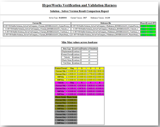
Figure 16. -
Click the first column of the table to open a new graphics window.
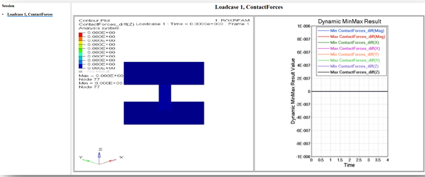
Figure 17.In the image above, the left window shows a diff contour (Current-Reference) and the right window shows a diff plot in HyperGraph.
In case any difference is greater than the tolerance, it is indicated with the label Fail. Otherwise, it is labeled Pass.
Solver Version Results Comparison (HyperView Option or HyperView Interactive )
-
From the Solution tab, select the Solver
version result comparison tab.
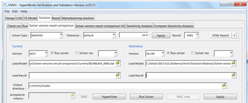
Figure 18. -
Under Current, in the Load Model field, click the file browser icon, , to load
the BOXBEAM_0000.rad file, located in
..\tutorials\hvvh\Solution\Radioss\Solver-versions-result-comparison\Current\.
-
Under Reference, in the Load Model field, click to load
the BOXBEAM_0000.rad file, located in
..\tutorials\hvvh\Solution\Radioss\Solver-versions-result-comparison\Reference\.
-
In the Output directory field, click to
select an output directory.
-
Click Run Solver.
After the solver run, the A001 results are loaded in the Load Result option.
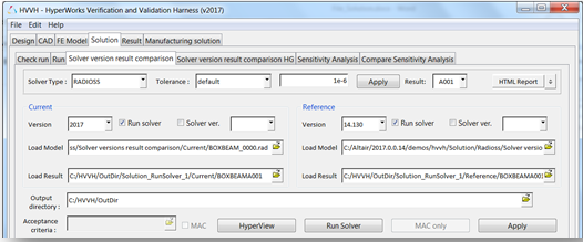
Figure 19. -
Display the results.
- In the first window, select a region of interest (element, node, component level) and create a contour.
- Run the command ::Displaycontour (reference result contour is also loaded for the selected region).
- Run a command to apply a user-defined tolerance for the data type selected ::Applytolerance (otherwise, use the default tolerance).
- Run the command ::Diffcontour. Difference contour result are displayed in another window for the selected data types only and are also plotted.
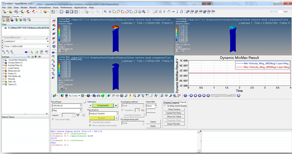
Figure 20.The first window displays the current model and result, and the second window displays the reference model and result.
The third window displays the difference in the contour values. If the difference is greater than the tolerance, it is indicated as Fail. Otherwise, displays Pass.
The fourth window displays the actual diff plots in HyperGraph.
The data type can be changed and any individual component result can be compared. Tolerance values can be reset to any value and result comparison.
- Comparison for region of interest:
- Part of the model (by window, by component, set of elements, and so on) can be selected in the first window. Using APIs as mentioned above, results can be compared ONLY for the selected region.
Solver Version Result Comparison HyperGraph
In this step, you will compare results from different solver versions ( Radioss or OptiStruct) using HyperGraph.
-
Select the Solution tab, then the Solver
version result comparison HG tab.
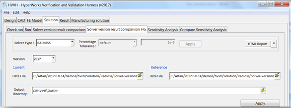
Figure 21. -
Under Current, for Data File, click the icon to
load the
..\tutorials\hvvh\Solution\Radioss\Solver-versions-result-comparison-HG\Current_BOXBEAMT01
file.
-
Under Reference, for Data File, click the icon to
load the
..\tutorials\hvvh\Solution\Radioss\Solver-versions-result-comparison-HG\Reference_BOXBEAMT01
file.
-
In the Output directory field, click to
select an output directory.
-
Click Apply.
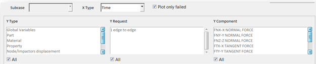
Figure 22. -
Select each All and click the second Apply.
Any combination of the Y-Type, Y Request, and Y Component can be selected for comparison.
In this example, the solver result for the same model with slightly different Boundary conditions are picked to show the difference in the results so that they are visible in the graphs of the report.
Results comparison of the current results and reference plot results are generated.
In the Messages window, the run details are displayed along with the log file location.
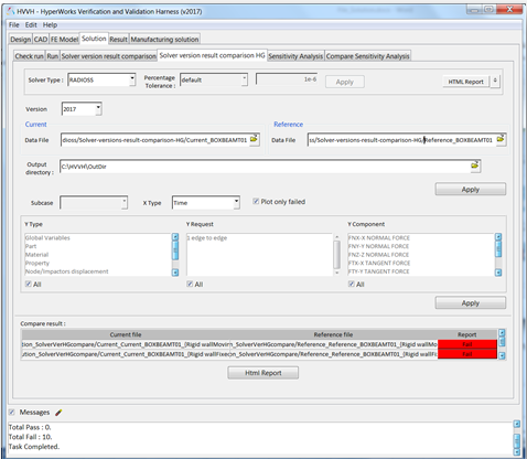
Figure 23. -
Click HTML Report to open the report.
Comparison of different Types, Requests, and Components (TRC) are available.
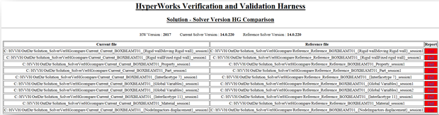
Figure 24.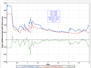
Figure 25.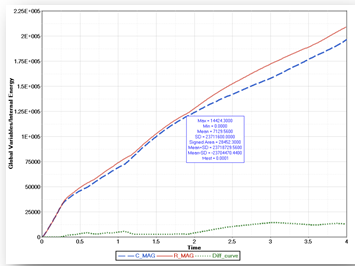
Figure 26.
Sensitivity Analysis
-
From the Solution tab, select the Sensitivity
Analysis tab.
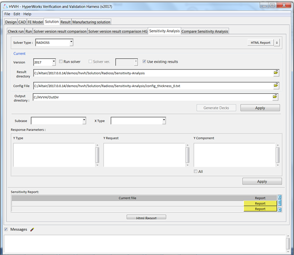 Figure 27.
 -
In the Result Directory field, click the file browser icon, , to load
the Sensitivity-Analysis file, located in
..\tutorials\hvvh\Solution\Radioss\Sensitivity-Analysis.
-
In the Config File field, click to load
the config_thickness_0.txt file, located in
..\tutorials\hvvh\Solution\Radioss\Sensitivity-Analysis\.
This file is used to set different seed values for the sensitivity analysis.
-
In the Output directory field, click to
select an output directory.
-
Click Apply.
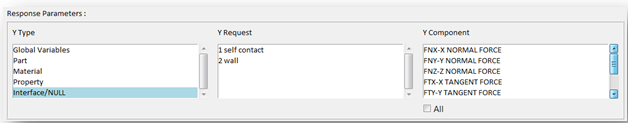
Figure 28. -
Under Response Parameters, select TRCs for the sensitivity study and click
Apply.
The sensitivity report is generated. In the Messages window, the run details and the log file location are displayed.
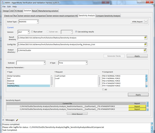
Figure 29.
Compare Sensitivity Analysis
Compare results from different solver versions using Sensitivity Analysis.
-
From the Solutions tab, select the Compare
Sensitivity Analysis tab.
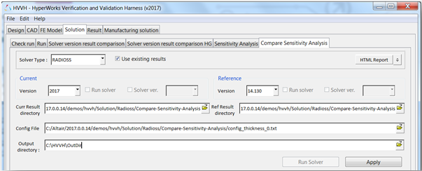
Figure 30. -
In the Current Result Directory field, click the file browser icon, , to load
the Compare-Sensitivity-Analysis file, located in
..\tutorials\hvvh\Solution\Radioss\.
-
In the Reference Result Directory field, click to load
the Compare-Sensitivity-Analysis, located in
..\tutorials\hvvh\Solution\Radioss\ file.
-
In the Config File field, click to load
the config_thickness_0.txt file, located in
..tutorials\hvvh\Solution\Radioss\Compare-Sensitivity-Analysis\.
-
In the Output directory field, click to
select an output directory.
-
Click Apply.
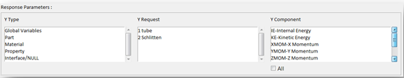 Figure 31.
 -
Select each All under the Type, Request, and Component
(TRC) windows. Click the second Apply button.
The sensitivity report is generated for comparison across two versions. In the Messages window, the run details are displayed along with the log file location.
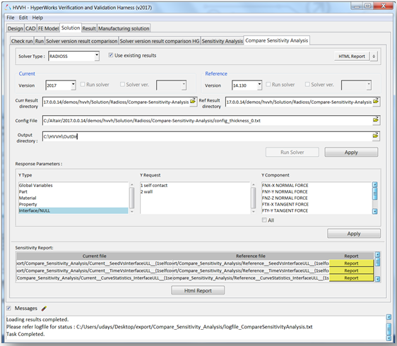
Figure 32. -
Click HTML Report to open the sensitivity report.
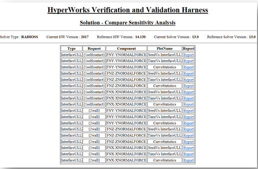
Figure 33.In the HTML report for one TRC, there will be two reports. For each of the solver results from different solver versions, the results are extracted and plotted for comparison.- Seed Vs TRC
- This is a scattered plot, showing sensitivity for each seed value. Using this sensitivity corridor, the variations across different seed vales for results from two solver versions can be determined.
- Time Vs TRC
- This shows Time History (TH) plots for the current and reference files and their diff curve.
- Curve Statistic
-
- Envelop of all curves (Max, Min, Mean, SD, Mean+SD, and Mean-SD).
- Statistical curves (Max, Min, Mean, SD, Mean+SD, and Mean-SD).
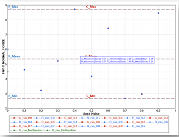
Figure 34.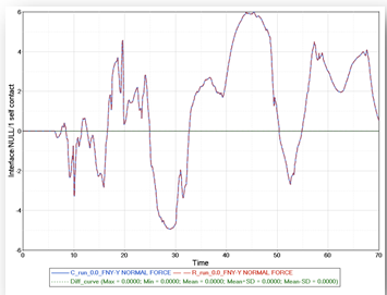
Figure 35.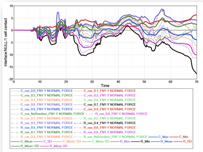
Figure 36.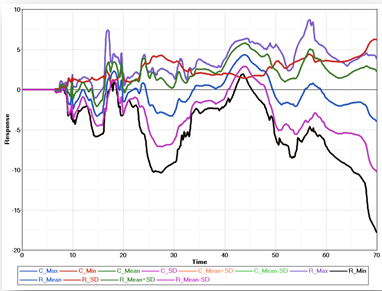
Figure 37.