Mesh Overview
The basis for any numerical analysis is solving the governing equations over a set of discrete volumes that enclose the physical domain. Mesh generation or grid generation is the process of generating such discrete volumes (elements) of the geometry.
The conservation equations of flow integrated over these discrete volumes is the basis of CFD. The accuracy of the solution is affected by the quality of the grid. There are different shapes of the elements that can be used for CFD analysis. However, the following are some of the commonly used shapes.
2D Elements
 Figure 1. Triangles |
 Figure 2. Quadrilateral |
3D Elements
 Figure 3. Tetrahedron |
 Figure 4. Pyramid |
 Figure 5. Prism |
 Figure 6. Hexahedron |
- Structured Grids: These type of grids are characterized by simple regular connectivity of the nodes. Such types of mesh can be obtained using quadrilateral elements in 2D plane and hexahedron (brick) elements in 3D space. These meshes are highly efficient in computer memory usage because of their simple connectivity. Structured grids have better convergence but it is difficult to generate such meshes on complex geometries.
- Unstructured Grids: These type of grids are characterized by simple shapes in irregular connectivity. This type of mesh can be obtained using triangular elements in 2D plane and mostly tetrahedron in 3D planes. These meshes are easy to generate for complex geometries but are not efficient in computer memory usage because of explicit storage of connectivity of elements.
- Hybrid Grids: Hybrid grids are a mix of both structured and unstructured grids. The parts of geometry which are regular may have structured grids and the complex parts may have unstructured grids.
Mesh Quality
Since the mesh holds the key for convergence and accuracy of the solution it is important to evaluate the quality of mesh. The following are some of the quality metrics to determine the mesh quality.
where is the optimal volume for tetrahedron, is the optimal triangle area, is the actual tetrahedron volume or triangle area and is the circumsphere or circumcircle radius.
Skewness ranges from zero (for equilateral triangle and tetrahedron) to one. The lower the skewness, the better the convergence.
The aspect ration can range from 1 to . The smaller the aspect ratio the better the mesh quality is.
Although different numerical analysis have different requirements on the minimum mesh quality, AcuSolve is capable of dealing with the bad elements effectively. The only necessary requirement for AcuSolve is that all of the elements have a positive jacobian, that is, elements with positive volumes.
In the regions of the flow with large gradients, the mesh has to be fine enough to capture those sharp gradients. The boundary layer near the wall is one such region in the flow with large gradients. Hence the proper resolution of the boundary layer is important for accurate solutions. Finer mesh at the wall with tetrahedrons would require larger computation time. However, by exploiting the fact that at the wall gradients along the stream are less compared to the transverse gradients, it is advantageous to use high aspect ratio prism elements for boundary layer. To avoid inaccuracies due to abrupt change in mesh sizes the mesh size has to transition smoothly from fine mesh at boundary to much coarser mesh at the core. Hence, the boundary layer mesh size is gradually increased from boundary to the core by a ratio (>1) called Stretch ratio, to approximately match mesh size in the inner core.
where = friction velocity = , = shear stress at the wall, = density of the fluid, = kinematic viscosity of fluid and = first cell height from the boundary.

Figure 7. Solution Approximations on Larger y+

Figure 8. Solution Approximations on Smaller y+

Figure 9. Closer View of Boundary Layer with Smaller y+
With a higher y+ the approximation of numerical solution cannot capture the boundary layer well. However, with a smaller y+ the boundary layer is captured very well. Hence the y+ plays a significant role in solution for the near wall region.
To accurately capture the near wall effects, a sufficient number of elements need to be present inside the viscous sub layer (typically y+ < 10). However to reduce the computational efforts, the near wall sub layers are modeled using wall functions, which uses semi-empirical approximations for the viscous sub layer. The appropriate y+ values depends on the turbulence models used and the type of wall functions.
Meshing in AcuConsole
AcuConsole uses AcuMeshSim as the mesher. AcuMeshSim operates directly on the underlying CAD model. When it performs surface meshing, it actually queries the underlying CAD kernel to determine where the node should fall in parametric space on CAD face. This ensures precise representation of the CAD. The input CAD model must be a non-manifold model. A non-manifold model is created automatically when you import a CAD model into AcuConsole. The process used to create the non-manifold representation of the geometry resolves overlapping volumes, eliminates duplicate faces, knits surfaces to form solids (if directed to), and performs a union between adjacent components. In all cases, AcuMeshSim requires a clean CAD. This means that the geometry must not have unjoined edges, unattached surfaces, gaps between common edges of surfaces, invalid spline representations of faces, and so on.
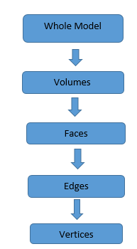
Figure 10. Hierarchy of CAD Model Entities for Meshing Parameters
Mesh attributes can be set on a global (whole model) and/or local (model entity) basis. An attribute specification applies to the closure of an entity, so if a size is specified on a model face the model edges and model vertices on the boundary of the face will inherit the same size specification. However, a separate size specification may be given for the edges and vertices in each case. If conflicting mesh sizes are specified, regardless of whether they are from the same type of mesh attributes or not, AcuMeshSim will pick the smaller of the resulting sizes.
All of the parameters related to the meshing can be viewed by clicking MSH in the Data Tree Manager.