Auto Calibration
Automatically calibrate propagation models based on measurement data.
Some propagation models support the calibration of material properties and of clutter/land usage databases. The following diagram shows the basic procedure for the calibration of the propagation models.
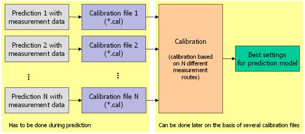
Figure 1. Procedure for the calibration of propagation models.
Calibration files can only be generated if measurement data is located within the prediction area or at the prediction points.
If the dominant path prediction model is used, the adaptive resolution management has to be disabled.
The calibration tool can be used to tune wave propagation models based on calibration files obtained during wave propagation predictions. The calibration tools can be started by selecting from the Computation menu. One or more calibration files can be added to the list.
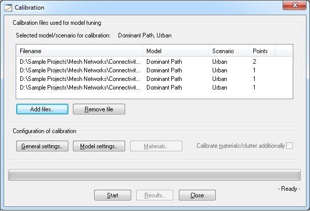
Figure 2. The Calibration dialog.
- Calibration Files Used for Model Tuning
- Files can be added by clicking on Add files or deleted by clicking on Remove file.
- Configuration of Calibration
-
- General Settings
- This allows the user to influence the selection of the measurement points, thus only points in a given power (dBm), path loss (dB) or distance (m) range will be considered.
- Model Settings
- The ranges of the model parameters can be defined here. As larger the range is, as longer the calibration will take. The model parameters depend on the selected propagation model, thus each model offers individual model parameters. The model parameters for the dominant path model are shown in Figure 3.
- Materials
- Depending on the propagation model the material database or the clutter/land usage database can also be calibrated.
- Start
- Starts the calibration computation. The current progress is displayed in a progress bar.
- Results
- After the calibration process has finished, the calibration results can be displayed.
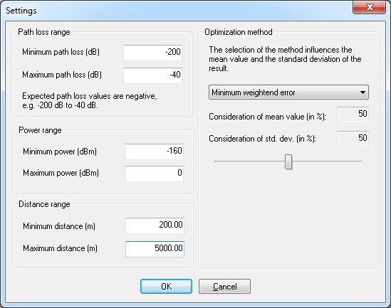
Figure 3. The Settings dialog - model parameters for the dominant path model.
- Minimum mean squared error:
The goal of the optimization is to achieve a minimum mean squared error. The standard deviation is not considered and thus might be larger.
- Minimum standard deviation:
The goal of the optimization is to achieve a minimum standard deviation. The mean error is not considered and thus might be larger.
- Minimum weighted error:
The goal of the optimization is to find the best combination of minimum mean error and minimum standard deviation. The weighting between mean error and standard deviation can be adapted by the user.
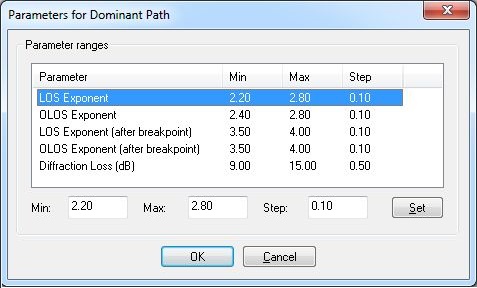
Figure 4. The Parameters for Dominant Path dialog.
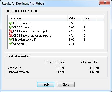
Figure 5. The Results for Dominant Path Urban dialog.
The statistical evaluation gives information about mean value and standard deviation from measurements to predictions before and after the calibration. Depending on the optimization method different results can be obtained.