Static Solution by Explicit Time Integration
Explicit algorithms are very useful for modeling a dynamic simulation. However, they cannot model a quasi-static or static simulation as easily. This is due to the fact that in an explicit approach, first the nodal accelerations are found by resolving the equilibrium equation at time . Other DOFs are then computed by explicit time integration. This procedure implies that the nodal acceleration must exist; however, some numerical methods may be employed for the simulation of a static process.
Slow Dynamic Computation
The loading is applied at a rate sufficiently slow to minimize the dynamic effects. The final solution is obtained by smoothing the curves.
In case of elasto-plastic problems, one must minimize dynamic overshooting because of the irreversibility of the plastic flow.
Dynamic Relaxation or Nodal Damping (/DYREL)
and
Where, is the relaxation coefficient whose recommended value is 1. is less than or equal to the highest period of the system. These are the input parameters used in /DYREL option.
Energy Discrete Relaxation
This empirical methodology consists in setting to zero the nodal velocities each time the Kinetic Energy reaches a maximum.
The loading is applied at a rate sufficiently slow to minimize the dynamic effects. The final solution is obtained by smoothing the curves.
In case of elasto-plastic problems, one must minimize dynamic overshooting because of the irreversibility of the plastic flow.
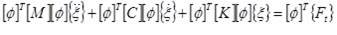
Rayleigh Damping (/DAMP)
Where, and are the pre-defined constants. In modal analysis, the use of a proportional damping matrix allows to reduce the global equilibrium equation to n-uncoupled equations by using an orthogonal transformation.
- The ith natural frequency of the system
- The ith damping ratio
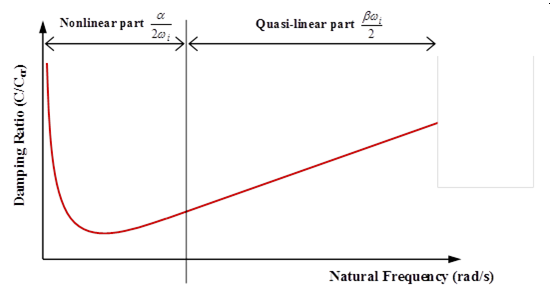
Figure 1. Rayleigh Damping Variation for Natural Frequencies
The three approaches available in Radioss are Dynamic Relaxation (/DYREL), Energy Discrete Relaxation (/KEREL) and Rayleigh Damping (/DAMP). Refer to Example Guide for application examples.
The loading is applied at a rate sufficiently slow to minimize the dynamic effects. The final solution is obtained by smoothing the curves.
In case of elasto-plastic problems, one must minimize dynamic overshooting because of the irreversibility of the plastic flow.
Acceleration Convergence
For every method, an acceleration of the convergence to the static solution is desirable. The constant time step is one of the more usual methods. In fact, in quasi-static analysis, the duration of the study is proportional to the maximum period of the structure. The total number of computation cycles is then proportional to the ratio .
- Largest period of the structure
- Time step
The number of time steps necessary to reach the static solution is minimal if all the elements have the same time step. An initial given time step can be obtained by increasing or decreasing the density of each element. The constant nodal time step option ensures a homogenous time step over the structure. However, in usual static problems the change is expected to be small, but one may think of increasing the density of the element which gives the critical time step in such a way that .