Static Solution by Implicit Time-Integration
The static behavior of many structures can be characterized by a load-deflection or force-displacement response. If the response plot is nonlinear, the structure behavior is nonlinear. From computational point of view the resolution of a nonlinear problem is much more complex with respect to the linear case. However, the use of relatively recent resolution methods based on sparse iterative techniques allows saving substantially in memory.
Linear Static Solver
A linear structure is a mathematical model characterized by a linear fundamental equilibrium path for all possible choices of load and deflection variables.
- The response to different load systems can be obtained by superposition,
- Removing all loads returns the structure to the reference position.
- Perfect linear elasticity for any deformation,
- Infinitesimal deformation,
- Infinite strength.
Despite of obvious physically unrealistic limitations, the linear model can be a good approximation of portions of nonlinear response. As the computational methods for linear problems are efficient and low cost, Radioss linear solvers can be used to find equilibrium of quasi-linear systems. The Preconditioned Conjugate Gradient method is the iterative linear solver available in Radioss. The algorithm enables saving a lot of memory for usual application of Radioss as a sparse storage method is used. This means that only the non-zero terms of the global stiffness matrix are saved. In addition, the symmetry property of both stiffness and preconditioning matrices is worthwhile to save memory.
The performance of conjugate gradient method depends highly to the preconditioning method. Several options are available in Radioss using the card /IMPL/SOLV/1. The simplest method is a so-called Jacobi method in which only the diagonal terms are taken into account. This choice allows saving considerable memory space; however, the performance may be poor. The incomplete Choleski is one of the best known effective preconditioning methods. However, it can result in negative pivots in some special cases even if the stiffness matrix is definite positive. This results a low convergence of PCG algorithm. The problem can be resolved by using a stabilization method. 1 Finally, the Factored Approximate Inverse method may be the best choice which is used by default in Radioss.
Nonlinear Static Solver
As explained in the beginning of this chapter, a nonlinear behavior is characterized by a nonlinear load-deflection diagram called path. The tangent to an equilibrium path may be formally viewed as the limit of the ratio force increment on displacement increment. This is the definition of a stiffness or more precisely the tangent stiffness related to a given equilibrium state. The reciprocal ratio is called flexibility. The sign of the tangent stiffness is closely associated with the stability of an equilibrium state. A negative stiffness is necessary associated with unstable equilibrium. A positive stiffness is necessary but not sufficient for stability.
Equation 3 can handle the solution of the nonlinear problem when an incremental method is used. The solution methods are generally based on continuous incremental and corrective phases. The most important class of corrective methods concerns the Newton-Raphson method and its numerous variants as modified, modified-delayed, damped, quasi and so forth. All of these Newton-like methods require access to the past solution. In the following section the conventional and modified Newton methods under general increment control are studied.
Newton and Modified New Methods
Several techniques are available to resolve Equation 5. In some situations, the parameter is fixed, and the equations are resolved to determine n components of in order to verify Equation 5. In this case, the technique is called load control method. Another technique called displacement control consists in fixing a component of and searching for and 'n-1' other components of displacement vector . A generalization of displacement control technique will enable to imply several components of displacement vector by using an Euclidian norm. The method is called arc-length control and intended to enable solution algorithms to pass limit points (that is, maximum and minimum loads). The techniques making possible to obtain the load-deflection curve by finding point by point the solution are called piloting techniques.
as and:
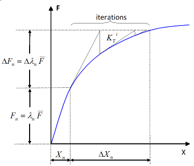
Figure 1. Standard Newton-Raphson Resolution in the Case of Load Control Technique
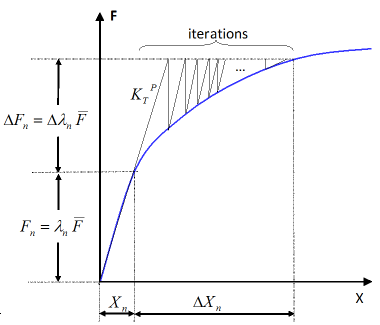
Figure 2. Modified Newton-Raphson Resolution in the Case of Load Control Technique
However, it is possible to save computation time which depends on the size of the problem and on the degree of the nonlinearity of the problem. The method is called modified Newton-Raphson which is based on the conservation of the tangent matrix for all iterations (Figure 2). This method can also be combined with the acceleration techniques as line-search explained in Line Search Method to Optimize the Resolution.
The convergence criteria may be based on Euclidian norm of residual forces, residual displacements or energy where an allowable tolerance is defined.
Line Search Method to Optimize the Resolution
Where, is obtained to minimize the total potential energy or to satisfy the principle of virtual works. The techniques to determine use often a Raleigh-Ritz procedure with only one unknown parameter.
For all kinematical acceptable
for all
The coefficients , , and can be expressed in terms of displacements and the increment of displacements .
Arc Length Method
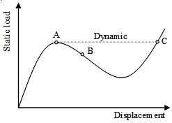 (a) Snap-through |
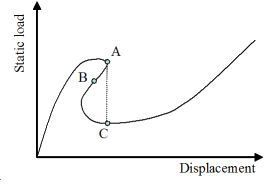 (b) Snap-backs |
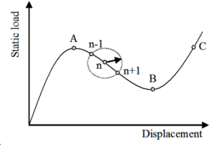 (c) Arc-length method: intersection of the equilibrium branch with the circle about the last solution |
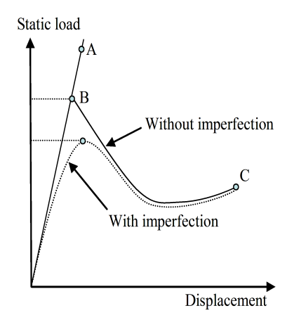 (d) Buckling with or without imperfections |
The tracing of equilibrium branches are quite difficult. In arc-length method, instead of incrementing the load parameter, a measure of the arc length in the displacement-load parameter space is incremented. This is accomplished by adding a controlling parameter to the equilibrium equations.
With:
;
;
In each of the Newton-Raphson iterations, Equation 20 must be resolved to select a real root. If there is no root, should be reduced. The most closed root to the last solution is retained in the case of two real roots.
Table 1(c) illustrates the intersection of the equilibrium branch with the circle about the last solution.