Shell Elements
Shell Elements (/PROP/SHELL)
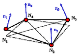
A shell is defined by a curved mid-surface and a thickness h, which is supposed to be very small compared to the two other dimensions. A shell element is the most common element; a full car crash model is made of at least 90% shell elements.
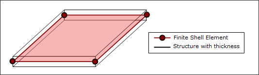
Figure 1. Shell Element
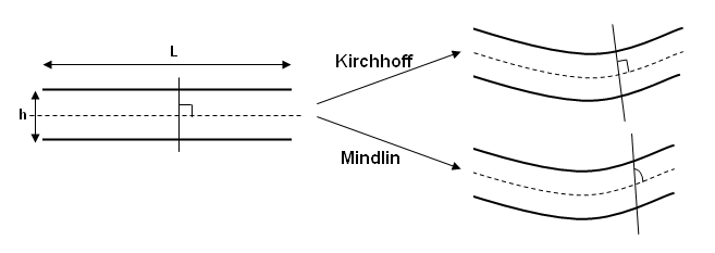
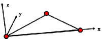
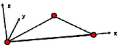
Figure 2. Shell Models
Even if the Kirchhoff model is less accurate, if the ratio L/h is greater than 20, the statements made by Kirchhoff are correct; but if the ratio L/h is between 10 and 20, the assumption stating that a plane orthogonal to the mid-plane remains orthogonal during the deformation is no longer valid, and the Mindlin plate model must be considered in which transverse shear strain is taken into account. In Radioss, under-integrated shell elements (both 4-node and 3-node shell) are based on Mindlin assumptions. There is no specific formulation that enables to offset the mid-plane of the element away from the nodes; therefore, it is very important to discretize structures with thin walls on the mid-surface.
| Mesh | Element Name | Number of Integration Points | Hourglass Formulation | Comments |
|---|---|---|---|---|
 |
BT
(Classic Q4) |
1 | Four types based on penalty method | Constant normal
vector Hourglass formulations types 3 and 4 are much better than type 1 - used by default |
 |
QEPH | 1 | Physical stabilization | Normal vectors at
nodes No hourglass energy in output |
 |
QBAT | 2x2 | Fully-integrated element | Normal vectors at
nodes No hourglass energy |
 |
C0 | 1 | --- | Flat facet
element No hourglass energy |
 |
DKT18 | 3 | --- | Kirchhoff shell
(thin shell only) Higher t/L, lower the time step |
 |
S3N6 | 1 | --- | Kirchhoff shell
(thin shell only) No rotational DOF Rotation of the sides is determined with the help of vertical displacements in neighbors |
- The BT element is simple, efficient and has a low cost. As it is under-integrated, the element is not very sensitive to the mesh quality and can be used for the case of coarse mesh.
- For cases of Quasi-Static Analysis, fine mesh, warped surface and buckling, it is advisable to use QEPH or QBAT elements.
- QBAT is the most accurate element in Radioss. However, as it is fully-integrated, it costs two to three times more than a BT element.
- QEPH is the best compromise between cost and quality. Generally, it costs no more than 15% of a BT element and the results obtained by this element are close to those of QBAT.
- Triangles are not recommended. A C0 element is too stiff and DKT18 comes with a high cost. The number of total triangles in a mesh is generally limited to 5% to ensure a good quality.
- The S3N6 element has as good a behavior in bending as DKT18. It can also be used for some special applications, such as stamping simulations.
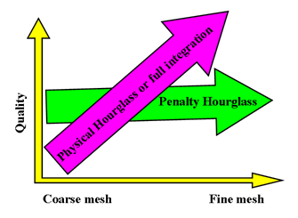
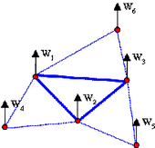
Figure 3. Use of Shell Formulations for Different Meshes
Integration through Thickness
In an elastic shell, the normal stress variation through the thickness is linear; therefore, the internal energy can be obtained by analytical integration. In case of plasticity, the stress distribution becomes nonlinear and a minimum of three integration points are required to take the nonlinearity into account. The nonlinear distribution of stress can be approached by measuring values at some added integration points. The quality of internal energy estimation depends on the number of integration points and the cost. A good compromise between cost and quality can be found, taking into account, material nonlinearity, thickness and bending rate. The number of integration points can be increased up to 10 in Radioss V5x. Using five integration points will provide better results; especially if the thickness is greater than 2mm, but the increase in CPU time is not negligible. To emulate a membrane element with no bending or transverse shear, it is enough to use only one integration point. For an elastic material (LAW1) due to the analytical computation, the option is ignored.
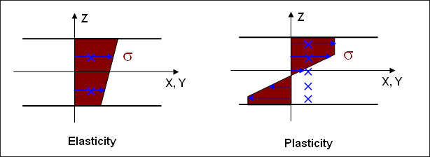
Figure 4. Normal Stress Distribution in a Section a Shell
One way to get accurate results with a low CPU cost is to use the global integration. It consists in the transformation of von Mises plasticity criteria, in a so-called Iluyshin criteria, where the stress components at integration points are replaced by internal forces (N, M, T, etc.).
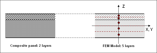
Figure 5. Layers Definition for Composite to Set the Number of Integration Points
Iterative Plastic Projection
In plasticity computation, two fundamental assumptions must be satisfied. First, the stress in the plastic region must verify the plasticity criteria (for example, von Mises criteria). Second, in the principal stresses space is the direction (), due to work hardening is normal to the yield surface.
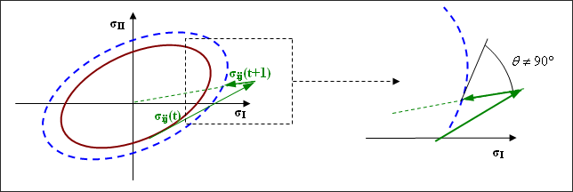
Figure 6. Radial Return
Thickness Variation
By default, shell thickness is supposed constant during shell deformation. Initial thickness is used to compute strains and to integrate stresses, but the thickness variation is still computed for post-processing reasons. If a variable thickness (Ithick =1) is used, true thickness is computed not only for post-processing, but also for strain computation and stresses integration.
Comments
- For accurate results, especially when necking or spring back, it is strongly recommended to use iterative plastic projection and thickness variation.
Element Option Guidelines
| Applications | Material | Property | Hourglass | Number of Integration Points | Thickness | Plasticity |
|---|---|---|---|---|---|---|
| Basic crash | 2 | 1 | 1 | 0 (global) | Constant | Radial |
| Crash with trapezoidal wrapped shells and with global rotation | 2 | 1 | 3(c) or QEPH | 0 (global) | Constant | Radial |
| Crash with spring back medium accuracy | 2/36 | 1 | 1 | 3 | Constant | Iteration |
| Crash with spring back high accuracy | 2/36 | 1 | 3(c) or QEPH | 3 | Variable | Iteration |
| Crash with material failure ductile failure | 2/36 (a) | 1 | 1 | 5 | Variable | Iteration |
| High quality crash | 2/36 (a) | 1 | 3(c) or QEPH | 5 | Variable | Iteration |
| Crash with material failure brittle failure | 27 | 11 | 1 | 3/5 | Variable | Iteration |
| Windshield | 27 | 11 | 1 | 3+1+3(b) | Variable | Iteration |
| Membrane or Fabric | 1/2/19/36 | 1 | 1 | 1 | cst/var | rad/iter |
| Composite | 25 | 9/10/11 | 1 | 1 to 30 | not used | not used |
| Model with local hourglass excitation | 2/... | 1 | 3(c) or QEPH | 0/3/5 | ||
| Model with low plasticity and low velocities | 2/... | 1 | 3(c) or QEPH | 3/5 |
- With variable thickness and iterative plasticity it is possible to model necking failure. The material hardening must be accurate.
- For glass, plastic, and glass windshield (3 glass layers, 1 plastic layer and 3 glass layers). Less accuracy, 2+1+2 can also be used. For more complex glass plastic windshields, more layers can be used.
- If elastoplastic hourglass (3) is used, it is recommended to use 0.1 for hm and hf and default for hr.