Modeling Tools

Skew and Frame (/SKEW & /FRAME)

Skews and frames are used to define local directions.

These directions can be used to apply:
  • Boundary conditions
  • Concentrated load
  • Fixed velocity
To define:
  • Rigid link orientation
  • Rigid body added inertia frame
  • General spring reference frame
  • Beam type spring initial reference frame
  • Nodal time history output frame
Two reference definitions are available in Radioss:
Skew reference
It is a projection reference to define the local quantities with respect to the global reference. In fact, the origin of the skew remains at the initial position during the motion even though a moving skew is defined. In this case, a simple projection matrix is used to compute the kinematic quantities in the reference.
In Figure 1, imposed velocity is applied in Y direction. In /IMPVEL, skew is used. Then the imposed velocity is computed in the Y axis of global coordinate system and then projected onto the Y’ axis of local skew reference.
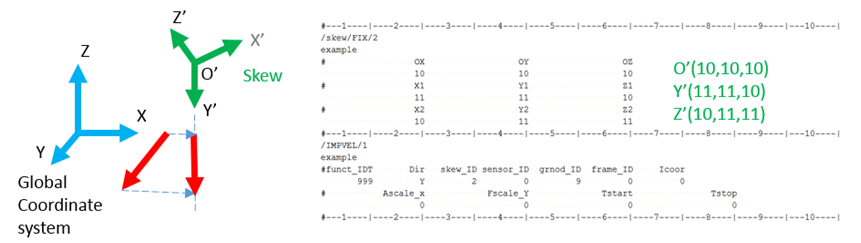

Figure 1. Skew Example
Frame reference
It is a mobile or fixed reference. The quantities are computed with respect to the origin of the frame which may be in motion or not depending on the kind of reference frame. For a moving reference frame, the position and the orientation of the reference vary in time during the motion. The origin of the frame defined by a node position is tied to the node.
Frame measures relative motion whereas skew measures global motion and projects it to skew. Only few options use frame like imposed velocity, TH/NODE and others use skew.
In Figure 2, rotational velocity is applied around Z axis. In /LOAD/CENTRI, frame is used. Then rotational velocity is around Z’ axis of frame reference not in Z axis of global coordinate system anymore.


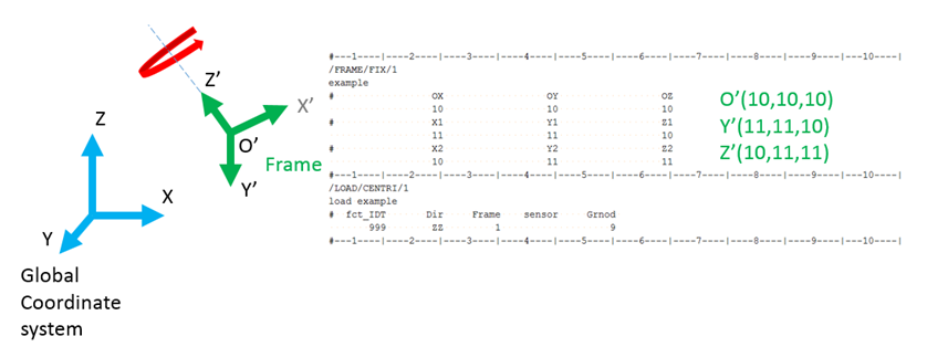
Figure 2. Frame Example

Sections (/SECT)

A section is used to measure the force, moment, and energy which are passing through a set of elements and nodes. The section displacements can also be saved to a file and used as imposed displacements in a smaller cut section model.

To define the section, the following are required:
  • A group of nodes and groups of elements. The nodes and elements can be selected by a user in /SECT. They can also be automatically selected by defining a section cut using /SECT with frame_ID, /SECT/PARAL, or /SECT/CIRCLE.
  • A local output system defined by selecting 3 points
  • A reference point to compute forces and moment


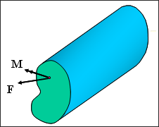
Figure 3. Definition of a Section for an Oriented Solid

Section Cutting Plane

In /SECT, the cutting plane is infinite and is defined by a group of elements and a group of nodes. The elements and nodes can be user-defined and should be along one row, if possible.

It is recommended to select all the nodes on one side of the element section.


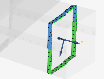
Figure 4. Elements and Nodes Selected Manually
Alternatively, the section cut can be defined using a local system. The local system /FRAME/MOV is defined by picking three nodes on the section cut. In this case, the element groups contain all the elements in the area of the section, and the node group in /SECT is not used. The nodes and elements on the xy plane of the local system are automatically selected for the section calculation. The cutting plane is the xy plane of the local system.


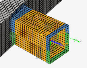
Figure 5. Element Group (in orange) defined for a section cut defined using a local system
The nodes and elements that lie on the section cut are then output in the Starter output file.
       NUMBER OF NODES. . . . . . . . . .        40
        NODES:
      6062      6064      6055      6074      6076      5895      6078      6173      6166      6136
      6174      6181      6182      6219      6210      6220      6227      6228      6359      6358
  ...

        NUMBER OF SHELL ELEMENTS . . . . .        43
   SHELL      N1      N2      N3      N4
      5819         0         1         1         0
      5820         0         1         1         0
      5826         0         0         1         0
      5839         0         1         1         0
   ...
In /SECT/PARAL, the cutting parallelogram is defined by three points M, M1, and M2 which define the two lines of the parallelogram. The element groups in the defined section should contain all the elements in the area of the parallelogram section. The nodes and elements used in the section calculation are automatically selected and output in the Starter output file, as shown previously for /SECT when a local system is used.


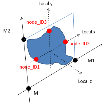
Figure 6. /SECT/PARAL Definition
In /SECT/CIRCLE, the cutting disk is defined by a point M, radius, and a normal vector. The element groups in the defined section should contain all the elements in the area of the circle section. The nodes and elements used in the section calculation are automatically selected and output in the Starter output file, as shown previously.


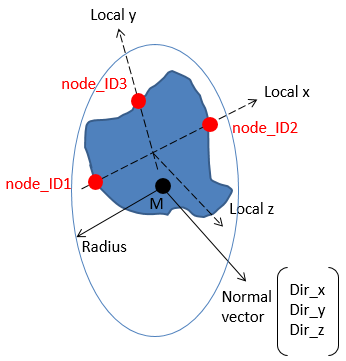
Figure 7. /SECT/CIRCLE Definition

All section types can cut solid, shell, truss, beam, and spring elements. Contact interfaces can also be selected.

When using /SECT with frame_ID, /SECT/PARAL, or /SECT/CIRCLE the nodes used for the section calculation will on the +z side of the selected elements. Since these nodes are automatically defined, the element groups can be defined by part and; thus, will not need to be redefined, if the part is re-meshed.

Local System of Cutting Plane

A local system must be defined to compute the force and moment from the section.

In all three section types (/SECT, /SECT/PARAL, and /SECT/CIRCLE), three nodes must be selected to define the local system used for the section output. These three nodes should be nodes on the section plane so their position is updated when the section moves. The nodes node_ID1, node_ID2, and node_ID3 define the local system as:
  • Nodes node_ID1 and node_ID2 define the local x-axis of the section.
  • Nodes node_ID1, node_ID2, and node_ID3 define the local plane xy of the section.
  • The local y-axis is defined by projecting node_ID3 perpendicular to the local x-axis.
  • The intersection of the local x- and y-axis is then the origin of the system.
  • The section normal is the local z-axis which is perpendicular to the xy plane.


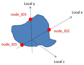
Figure 8. Section local system defined using nodes

When creating a /SECT in HyperMesh, these three nodes are automatically selected for the user. If they are manually selected, it is recommended to select nodes that belong to the group of nodes used in the section calculation. This will allow the local system to move as the section deforms.

Alternatively, in /SECT if the 3 nodes are not defined and instead a frame_ID is defined then the xy plane of the /FRAME/MOV is used as the local system. When defining the /FRAME/MOV it is recommended to use nodes that belong to the group of nodes used in the section calculation.

Force and Moment Computation

The section force is the sum of nodal force coming from the selected elements.

(1) F = f i MathType@MTEF@5@5@+= feaagKart1ev2aqatCvAUfeBSjuyZL2yd9gzLbvyNv2CaerbuLwBLn hiov2DGi1BTfMBaeXatLxBI9gBaerbd9wDYLwzYbItLDharqqtubsr 4rNCHbGeaGqiVu0Je9sqqrpepC0xbbL8F4rqGqFfpeea0xe9vq=Jb9 vqpeea0xd9q8qiYRWxGi6xij=hbba9q8aq0=yq=He9q8qiLsFr0=vr 0=vr0db8meaabaqaciGacaGaaeqabaWaaeaaeaaakeaacaWGgbGaey ypa0ZaaabqaeaacaWGMbWaaSbaaSqaaiaadMgaaeqaaaqabeqaniab ggHiLdaaaa@3D47@
The normal Force FN of the section is the component of section force in the normal direction and tangent force FT of the section is the component of section force in cutting plane.


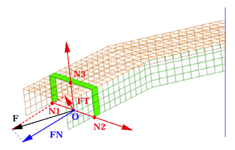
Figure 9. Normal section force and tangent section force in section
The section moment is the sum of nodal forces coming from the selected element multiplied by the distance to the local coordinate system center.(2) M = m i + O N i × f i MathType@MTEF@5@5@+= feaagKart1ev2aqatCvAUfeBSjuyZL2yd9gzLbvyNv2CaerbuLwBLn hiov2DGi1BTfMBaeXatLxBI9gBaerbd9wDYLwzYbItLDharqqtubsr 4rNCHbGeaGqiVu0Je9sqqrpepC0xbbL8F4rqGqFfpeea0xe9vq=Jb9 vqpeea0xd9q8qiYRWxGi6xij=hbba9q8aq0=yq=He9q8qiLsFr0=vr 0=vr0db8meaabaqaciGacaGaaeqabaWaaeaaeaaakeaacaWGnbGaey ypa0ZaaabqaeaacaWGTbWaaSbaaSqaaiaadMgaaeqaaaqabeqaniab ggHiLdGccqGHRaWkdaaeabqaaiaad+eacaWGobWaaSbaaSqaaiaadM gaaeqaaaqabeqaniabggHiLdGccqGHxdaTcaWGMbWaaSbaaSqaaiaa dMgaaeqaaaaa@4731@


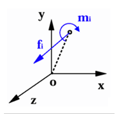
Figure 10. Resultant of force and moment for a node
Moments are computed with respect to the section center defined by the parameter Iframe. Options for the output system center include local system origin, geometric center, center of gravity, and global system origin. The output system can be either the local system or the global system.


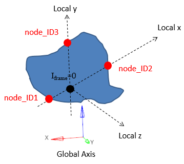
Figure 11. Iframe=0 Local system and origin used for section output


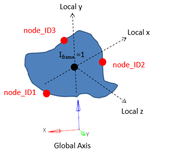
Figure 12. Iframe=1 Local system with the origin as the geometric center of the section


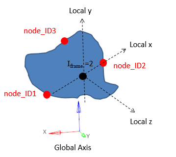
Figure 13. Iframe=2 Local system with the origin as the center of gravity of the section


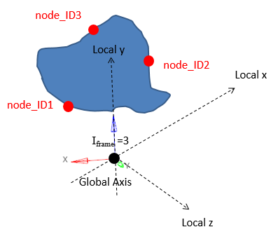
Figure 14. Iframe=3 Local system with the global origin as the center


Figure 15. Iframe=10 Global system with the center as the local system origin


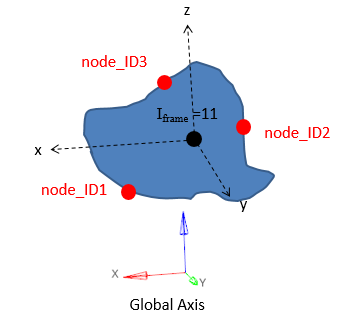
Figure 16. Iframe=11 Global system with the origin as the geometric center of the section


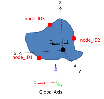
Figure 17. Iframe=12 Global system with the origin as the center of gravity of the section


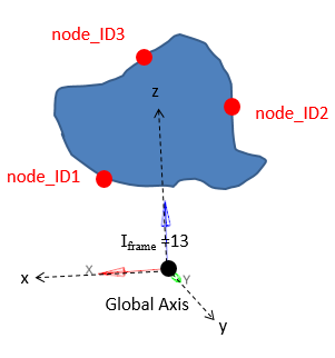
Figure 18. Iframe=13 Global system with the global origin as the center

Output of Section

Two types of section output are available.

First is the time history output /TH/SECTIO consisting of the sum of the force and moments acting on the section. The output can be in the global system or the local system with the most commons output being the variable groups, GLOBAL, LOCAL, and CENTER.

The second type of output is displacements and optional force and moment for every node in the section written to the section output data SC01 file. This file can then be read as an imposed displacement applied to a second cut section model. RD-E: 5400 Cut Methodology is an example of the cut section methodology that can be used. In this case, a full model is run with ISAVE=1 or 2 to save displacement and optionally the resultant section forces/moments in the file file_nameSC01.

Next, the second cut model (submodel) is created with a section defined using the option ISAVE=100 or 101 to read the displacement of the nodes the section file. The section’s local system defined by the three nodes node_ID1, node_ID2, and node_ID3 or frame_ID must be the same one used when saving the data (ISAVE=1 or 2) and reading the data (ISAVE=100 or 101).

If ISAVE=2 is used in the full model and ISAVE=101 is used in the cut model, then Radioss outputs the difference between resultant section forces and moments in full and cut model in the section (/TH/SECTIO).

To improve solution times and decrease memory needed, it is recommended to set ISAVE =0 if no cut modeling methodology is needed.

Filter

When reading and applying the displacements to a cut section model, the displacement can be filtered using an exponential moving average filter. For example, the filtered displacement in the x-direction would be:(3) x f =αx( t )+( 1α )x( tdt ) MathType@MTEF@5@5@+= feaagKart1ev2aaatCvAUfeBSjuyZL2yd9gzLbvyNv2CaerbuLwBLn hiov2DGi1BTfMBaeXatLxBI9gBaerbd9wDYLwzYbItLDharqqtubsr 4rNCHbGeaGqiVu0Je9sqqrpepC0xbbL8F4rqqrFfpeea0xe9Lq=Jc9 vqaqpepm0xbba9pwe9Q8fs0=yqaqpepae9pg0FirpepeKkFr0xfr=x fr=xb9adbaqaaeGaciGaaiaabeqaamaabaabaaGcbaGaamiEamaaBa aaleaacaWGMbaabeaakiabg2da9iabeg7aHjaadIhadaqadaqaaiaa dshaaiaawIcacaGLPaaacqGHRaWkdaqadaqaaiaaigdacqGHsislcq aHXoqyaiaawIcacaGLPaaacaWG4bWaaeWaaeaacaWG0bGaeyOeI0Ia amizaiaadshaaiaawIcacaGLPaaaaaa@4A38@
Where,
x f MathType@MTEF@5@5@+= feaagKart1ev2aaatCvAUfeBSjuyZL2yd9gzLbvyNv2CaerbuLwBLn hiov2DGi1BTfMBaeXatLxBI9gBaerbd9wDYLwzYbItLDharqqtubsr 4rNCHbGeaGqiVu0Je9sqqrpepC0xbbL8F4rqqrFfpeea0xe9Lq=Jc9 vqaqpepm0xbba9pwe9Q8fs0=yqaqpepae9pg0FirpepeKkFr0xfr=x fr=xb9adbaqaaeGaciGaaiaabeqaamaabaabaaGcbaGaamiEamaaBa aaleaacaWGMbaabeaaaaa@380A@
Filtered displacement
α MathType@MTEF@5@5@+= feaagKart1ev2aaatCvAUfeBSjuyZL2yd9gzLbvyNv2CaerbuLwBLn hiov2DGi1BTfMBaeXatLxBI9gBaerbd9wDYLwzYbItLDharqqtubsr 4rNCHbGeaGqiVu0Je9sqqrpepC0xbbL8F4rqqrFfpeea0xe9Lq=Jc9 vqaqpepm0xbba9pwe9Q8fs0=yqaqpepae9pg0FirpepeKkFr0xfr=x fr=xb9adbaqaaeGaciGaaiaabeqaamaabaabaaGcbaGaeqySdegaaa@3795@
Exponential moving average filtering constant
x ( t ) MathType@MTEF@5@5@+= feaagKart1ev2aaatCvAUfeBSjuyZL2yd9gzLbvyNv2CaerbuLwBLn hiov2DGi1BTfMBaeXatLxBI9gBaerbd9wDYLwzYbItLDharqqtubsr 4rNCHbGeaGqiVu0Je9sqqrpepC0xbbL8F4rqqrFfpeea0xe9Lq=Jc9 vqaqpepm0xbba9pwe9Q8fs0=yqaqpepae9pg0FirpepeKkFr0xfr=x fr=xb9adbaqaaeGaciGaaiaabeqaamaabaabaaGcbaGaamiEamaabm aabaGaamiDaaGaayjkaiaawMcaaaaa@3975@
Unfiltered displacement at the current time
x( tdt ) MathType@MTEF@5@5@+= feaagKart1ev2aaatCvAUfeBSjuyZL2yd9gzLbvyNv2CaerbuLwBLn hiov2DGi1BTfMBaeXatLxBI9gBaerbd9wDYLwzYbItLDharqqtubsr 4rNCHbGeaGqiVu0Je9sqqrpepC0xbbL8F4rqqrFfpeea0xe9Lq=Jc9 vqaqpepm0xbba9pwe9Q8fs0=yqaqpepae9pg0FirpepeKkFr0xfr=x fr=xb9adbaqaaeGaciGaaiaabeqaamaabaabaaGcbaGaamiEamaabm aabaGaamiDaiabgkHiTiaadsgacaWG0baacaGLOaGaayzkaaaaaa@3C44@
Displacement at the previous time step

Recommendations are:

α= 2πdt T MathType@MTEF@5@5@+= feaagKart1ev2aqatCvAUfeBSjuyZL2yd9gzLbvyNv2CaerbuLwBLn hiov2DGi1BTfMBaeXatLxBI9gBaerbd9wDYLwzYbItLDharqqtubsr 4rNCHbGeaGqiVu0Je9sqqrpepC0xbbL8F4rqqrFfpeea0xe9Lq=Jc9 vqaqpepm0xbba9pwe9Q8fs0=yqaqpepae9pg0FirpepeKkFr0xfr=x fr=xb9adbaqaaeGaciGaaiaabeqaamaabaabaaGcbaGaeqySdeMaey ypa0ZaaSaaaeaacaaIYaGaeqiWdaNaamizaiaadshaaeaacaWGubaa aaaa@3DE0@ for filtering -3dB

α= 2πdt 3T MathType@MTEF@5@5@+= feaagKart1ev2aqatCvAUfeBSjuyZL2yd9gzLbvyNv2CaerbuLwBLn hiov2DGi1BTfMBaeXatLxBI9gBaerbd9wDYLwzYbItLDharqqtubsr 4rNCHbGeaGqiVu0Je9sqqrpepC0xbbL8F4rqqrFfpeea0xe9Lq=Jc9 vqaqpepm0xbba9pwe9Q8fs0=yqaqpepae9pg0FirpepeKkFr0xfr=x fr=xb9adbaqaaeGaciGaaiaabeqaamaabaabaaGcbaGaeqySdeMaey ypa0ZaaSaaaeaacaaIYaGaeqiWdaNaamizaiaadshaaeaadaGcaaqa aiaaiodacaWGubaaleqaaaaaaaa@3EB8@ for filtering -6dB

Where,
T MathType@MTEF@5@5@+= feaagKart1ev2aqatCvAUfeBSjuyZL2yd9gzLbvyNv2CaerbuLwBLn hiov2DGi1BTfMBaeXatLxBI9gBaerbd9wDYLwzYbItLDharqqtubsr 4rNCHbGeaGqiVu0Je9sqqrpepC0xbbL8F4rqqrFfpeea0xe9Lq=Jc9 vqaqpepm0xbba9pwe9Q8fs0=yqaqpepae9pg0FirpepeKkFr0xfr=x fr=xb9adbaqaaeGaciGaaiaabeqaamaabaabaaGcbaGaamivaaaa@36D0@
Filtering period
dt MathType@MTEF@5@5@+= feaagKart1ev2aqatCvAUfeBSjuyZL2yd9gzLbvyNv2CaerbuLwBLn hiov2DGi1BTfMBaeXatLxBI9gBaerbd9wDYLwzYbItLDharqqtubsr 4rNCHbGeaGqiVu0Je9sqqrpepC0xbbL8F4rqqrFfpeea0xe9Lq=Jc9 vqaqpepm0xbba9pwe9Q8fs0=yqaqpepae9pg0FirpepeKkFr0xfr=x fr=xb9adbaqaaeGaciGaaiaabeqaamaabaabaaGcbaGaamizaiaads haaaa@37D9@
Model time step

The filtering period T = 10 Δ t MathType@MTEF@5@5@+= feaagKart1ev2aqatCvAUfeBSjuyZL2yd9gzLbvyNv2CaerbuLwBLn hiov2DGi1BTfMBaeXatLxBI9gBaerbd9wDYLwzYbItLDharqqtubsr 4rNCHbGeaGqiVu0Je9sqqrpepC0xbbL8F4rqqrFfpeea0xe9Lq=Jc9 vqaqpepm0xbba9pwe9Q8fs0=yqaqpepae9pg0FirpepeKkFr0xfr=x fr=xb9adbaqaaeGaciGaaiaabeqaamaabaabaaGcbaGaamivaiabg2 da9iaaigdacaaIWaGaeuiLdqKaamiDaaaa@3BAA@ is often used making α = 2 π 10 = 0.62832 MathType@MTEF@5@5@+= feaagKart1ev2aqatCvAUfeBSjuyZL2yd9gzLbvyNv2CaerbuLwBLn hiov2DGi1BTfMBaeXatLxBI9gBaerbd9wDYLwzYbItLDharqqtubsr 4rNCHbGeaGqiVu0Je9sqqrpepC0xbbL8F4rqqrFfpeea0xe9Lq=Jc9 vqaqpepm0xbba9pwe9Q8fs0=yqaqpepae9pg0FirpepeKkFr0xfr=x fr=xb9adbaqaaeGaciGaaiaabeqaamaabaabaaGcbaGaeqySdeMaey ypa0ZaaSaaaeaacaaIYaGaeqiWdahabaGaaGymaiaaicdaaaGaeyyp a0deaaaaaaaaa8qacaaIWaGaaiOlaiaaiAdacaaIYaGaaGioaiaaio dacaaIYaaaaa@42E3@ for a -3dB filter.