Materials

Different material tests could result in different material mechanic character.

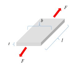
The typical material test for metal is tensile test. With this test strain-stress curve, yield point, necking point and failure point of material could be observed.

Engineer strain-stress curve could be generated by:(1)

σ_{e} = \frac{F}{S_{0}}

(2)

ε_{e} = \frac{Δ l}{l_{0}}

Where,

$S_{0}$: Section area in the initial state
$l_{0}$: Initial length

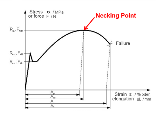
In this Force-elongation curve or engineer stress-strain curve, three points are important.

Yield point: where material begin to yield. Before yield you can assume material is in elastic state (the Young's modulus E could be measured) and after yield, material plastic strain which is non-reversible.
- Some material in this test will first reach the upper yield point (R_eH) and then drop to the lower yield point (R_eL). In engineer stress-strain curve, lower yield stress (conservative value) could be taken.
- Some material can not easily find yield point. Take the stress of 0.1 or 0.2% plastic strain as yield stress.
Necking point: where the material reaches the maximal stress in engineer stress-strain curve. After this point, the material begins to soften.
Failure point: where material failed.

R_m: Maximum resistance
F_max: Maximum force
R_eH: Upper yield level
R_eL: Lower yield level
A_g: Uniform elongation
A_gt: Total uniform elongation
A_t: Total failure strain

True stress-strain curve which is requested in most materials in Radioss, except in LAW2, where both engineer stress-strain and true stress-strain are possible to input material data.

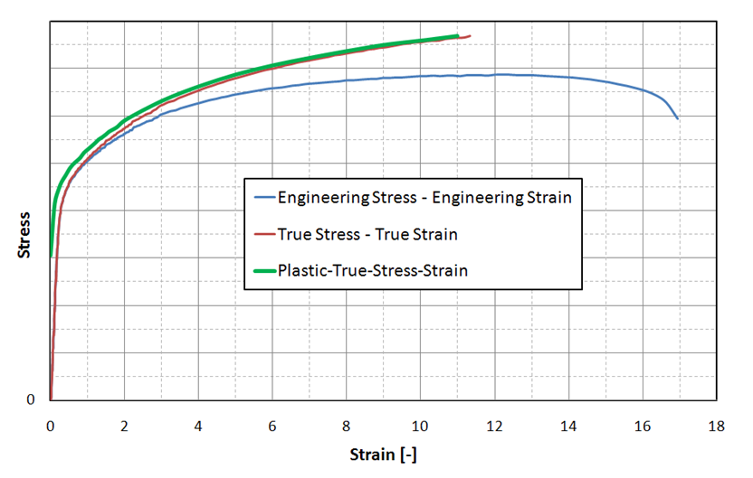
In Figure 3, find engineer stress-strain curve (blue) by using:(3)

σ_{t r} = σ_{e} exp (ε_{t r})

(4)

ε_{t r} = ln (1 + ε_{e})

The result is true stress-strain curve (red). Plastic true stress-strain curve is shown in green, which plastic strain begin from 0. This green plastic true stress-strain curve is what you need, as in LAW36, LAW60, LAW63, and so on.

The true stress-strain curve is valid until the necking point of the material. After the necking point, the material curve has to be defined manually for hardening. Using a different material law, Radioss will extrapolation the true stress-strain curve to 100%.

Linear extrapolation: If stress-strain curve is as function input (LAW36), then stress-strain curve is linearly extrapolated with a slope defined by the last two points of the curve. It is recommended that the list of abscissa value be increased to a value greater than the previous abscissa value.
Johnson-Cook: After necking point, Johnson-Cook hardening is one of the most commonly used to extrapolate the true stress-strain curve.(5)
$σ_{y} = a + b ε_{p}^{n}$

However, it may overestimate strain hardening for automotive steel, In this case, combination of swift-voce hardening is more accurate.
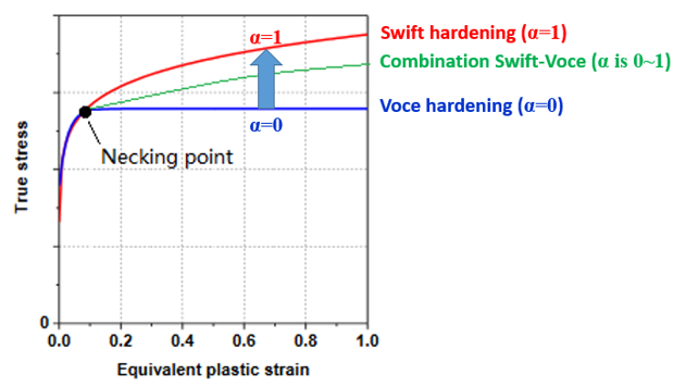
Swift and Voce: After necking point, use one of the following equations to extrapolate the true stress-strain curve.

Swift model

$σ_{y} = A {({\bar{ε}}_{p} + ε_{0})}^{n}$

$A$ and $n$ are positive.

Voce model

$σ_{y} = k_{0} + Q [1 - \exp (- B {\bar{ε}}_{p})]$

$k_{0}$ , $Q$ and $B$ are positive.

Combination of Swift and Voce model (LAW84 and LAW87)

$σ_{y} = α \underset{S w i f t \begin{matrix} \end{matrix} h a r d e n i n g}{\underset{︸}{[A {({\bar{ε}}_{p} + ε_{0})}^{n}]}} + (1 - α) \underset{V o c e \begin{matrix} \end{matrix} h a r d e n i n g}{\underset{︸}{{k_{0} + Q [1 - \exp (- B {\bar{ε}}_{p})]}}}$

Here, α is weight of Swift hardening and Voce hardening. Here one Compose script as example to fit the Swift hardening parameters

A

ε_{0}

n

and Voce hardening parameters

k_{0}

Q

B

with input stress-strain curve.