/FAIL/BIQUAD

In Radioss, /FAIL/BIQUAD is the most user-friendly failure model for ductile materials. It uses a simplified, nonlinear strain-based failure criteria with linear damage accumulation.

The failure strain is described by two parabolic functions calculated using curve fitting from up to 5 user input failure strains.

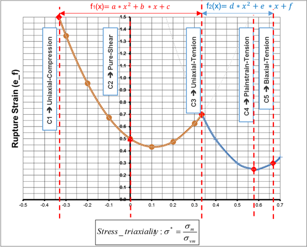
By default, /FAIL/BIQUAD (S-Flag=1) uses two parabolic curves to describe the plastic failure strain ε f MathType@MTEF@5@5@+= feaagKart1ev2aqatCvAUfeBSjuyZL2yd9gzLbvyNv2CaerbuLwBLn hiov2DGi1BTfMBaeXatLxBI9gBaerbd9wDYLwzYbItLDharqqtubsr 4rNCHbGeaGqiVu0Je9sqqrpepC0xbbL8F4rqGqFfpeea0xe9vq=Jb9 vqpeea0xd9q8qiYRWxGi6xij=hbba9q8aq0=yq=He9q8qiLsFr0=vr 0=vr0db8meaabaqaciGacaGaaeqabaWaaeaaeaaakeaacqaH1oqzda WgaaWcbaGaamOzaaqabaaaaa@3A26@ , as a function of stress triaxiality σ * MathType@MTEF@5@5@+= feaagKart1ev2aqatCvAUfeBSjuyZL2yd9gzLbvyNv2CaerbuLwBLn hiov2DGi1BTfMBaeXatLxBI9gBaerbd9wDYLwzYbItLDharqqtubsr 4rNCHbGeaGqiVu0Je9sqqrpepC0xbbL8F4rqGqFfpeea0xe9vq=Jb9 vqpeea0xd9q8qiYRWxGi6xij=hbba9q8aq0=yq=He9q8qiLsFr0=vr 0=vr0db8meaabaqaciGacaGaaeqabaWaaeaaeaaakeaacqaHdpWCda ahaaWcbeqaaiaacQcaaaaaaa@3A06@ . The two parabolic curves use:(1)
f 1 ( x )=a x 2 +bx+c MathType@MTEF@5@5@+= feaagKart1ev2aqatCvAUfeBSjuyZL2yd9gzLbvyNv2CaerbuLwBLn hiov2DGi1BTfMBaeXatLxBI9gBaerbd9wDYLwzYbItLDharqqtubsr 4rNCHbGeaGqiVu0Je9sqqrpepC0xbbL8F4rqGqFfpeea0xe9vq=Jb9 vqpeea0xd9q8qiYRWxGi6xij=hbba9q8aq0=yq=He9q8qiLsFr0=vr 0=vr0db8meaabaqaciGacaGaaeqabaWaaeaaeaaakeaacaWGMbWaaS baaSqaaiaaigdaaeqaaOWaaeWaaeaacaWG4baacaGLOaGaayzkaaGa eyypa0JaamyyaiaadIhadaahaaWcbeqaaiaaikdaaaGccqGHRaWkca WGIbGaamiEaiabgUcaRiaadogaaaa@4436@
(2)
f 2 ( x )=d x 2 +ex+f MathType@MTEF@5@5@+= feaagKart1ev2aqatCvAUfeBSjuyZL2yd9gzLbvyNv2CaerbuLwBLn hiov2DGi1BTfMBaeXatLxBI9gBaerbd9wDYLwzYbItLDharqqtubsr 4rNCHbGeaGqiVu0Je9sqqrpepC0xbbL8F4rqGqFfpeea0xe9vq=Jb9 vqpeea0xd9q8qiYRWxGi6xij=hbba9q8aq0=yq=He9q8qiLsFr0=vr 0=vr0db8meaabaqaciGacaGaaeqabaWaaeaaeaaakeaacaWGMbWaaS baaSqaaiaaikdaaeqaaOWaaeWaaeaacaWG4baacaGLOaGaayzkaaGa eyypa0JaamizaiaadIhadaahaaWcbeqaaiaaikdaaaGccqGHRaWkca WGLbGaamiEaiabgUcaRiaadAgaaaa@4440@
Where,
a MathType@MTEF@5@5@+= feaagKart1ev2aqatCvAUfeBSjuyZL2yd9gzLbvyNv2CaerbuLwBLn hiov2DGi1BTfMBaeXatLxBI9gBaerbd9wDYLwzYbItLDharqqtubsr 4rNCHbGeaGqiVu0Je9sqqrpepC0xbbL8F4rqGqFfpeea0xe9vq=Jb9 vqpeea0xd9q8qiYRWxGi6xij=hbba9q8aq0=yq=He9q8qiLsFr0=vr 0=vr0db8meaabaqaciGacaGaaeqabaWaaeaaeaaakeaacaWGHbaaaa@384E@ , b MathType@MTEF@5@5@+= feaagKart1ev2aqatCvAUfeBSjuyZL2yd9gzLbvyNv2CaerbuLwBLn hiov2DGi1BTfMBaeXatLxBI9gBaerbd9wDYLwzYbItLDharqqtubsr 4rNCHbGeaGqiVu0Je9sqqrpepC0xbbL8F4rqGqFfpeea0xe9vq=Jb9 vqpeea0xd9q8qiYRWxGi6xij=hbba9q8aq0=yq=He9q8qiLsFr0=vr 0=vr0db8meaabaqaciGacaGaaeqabaWaaeaaeaaakeaacaWGHbaaaa@384E@ , c MathType@MTEF@5@5@+= feaagKart1ev2aqatCvAUfeBSjuyZL2yd9gzLbvyNv2CaerbuLwBLn hiov2DGi1BTfMBaeXatLxBI9gBaerbd9wDYLwzYbItLDharqqtubsr 4rNCHbGeaGqiVu0Je9sqqrpepC0xbbL8F4rqGqFfpeea0xe9vq=Jb9 vqpeea0xd9q8qiYRWxGi6xij=hbba9q8aq0=yq=He9q8qiLsFr0=vr 0=vr0db8meaabaqaciGacaGaaeqabaWaaeaaeaaakeaacaWGHbaaaa@384E@ , d MathType@MTEF@5@5@+= feaagKart1ev2aqatCvAUfeBSjuyZL2yd9gzLbvyNv2CaerbuLwBLn hiov2DGi1BTfMBaeXatLxBI9gBaerbd9wDYLwzYbItLDharqqtubsr 4rNCHbGeaGqiVu0Je9sqqrpepC0xbbL8F4rqGqFfpeea0xe9vq=Jb9 vqpeea0xd9q8qiYRWxGi6xij=hbba9q8aq0=yq=He9q8qiLsFr0=vr 0=vr0db8meaabaqaciGacaGaaeqabaWaaeaaeaaakeaacaWGHbaaaa@384E@ , e MathType@MTEF@5@5@+= feaagKart1ev2aqatCvAUfeBSjuyZL2yd9gzLbvyNv2CaerbuLwBLn hiov2DGi1BTfMBaeXatLxBI9gBaerbd9wDYLwzYbItLDharqqtubsr 4rNCHbGeaGqiVu0Je9sqqrpepC0xbbL8F4rqGqFfpeea0xe9vq=Jb9 vqpeea0xd9q8qiYRWxGi6xij=hbba9q8aq0=yq=He9q8qiLsFr0=vr 0=vr0db8meaabaqaciGacaGaaeqabaWaaeaaeaaakeaacaWGHbaaaa@384E@ , and f MathType@MTEF@5@5@+= feaagKart1ev2aqatCvAUfeBSjuyZL2yd9gzLbvyNv2CaerbuLwBLn hiov2DGi1BTfMBaeXatLxBI9gBaerbd9wDYLwzYbItLDharqqtubsr 4rNCHbGeaGqiVu0Je9sqqrpepC0xbbL8F4rqGqFfpeea0xe9vq=Jb9 vqpeea0xd9q8qiYRWxGi6xij=hbba9q8aq0=yq=He9q8qiLsFr0=vr 0=vr0db8meaabaqaciGacaGaaeqabaWaaeaaeaaakeaacaWGHbaaaa@384E@
Parabolic coefficients
x MathType@MTEF@5@5@+= feaagKart1ev2aqatCvAUfeBSjuyZL2yd9gzLbvyNv2CaerbuLwBLn hiov2DGi1BTfMBaeXatLxBI9gBaerbd9wDYLwzYbItLDharqqtubsr 4rNCHbGeaGqiVu0Je9sqqrpepC0xbbL8F4rqGqFfpeea0xe9vq=Jb9 vqpeea0xd9q8qiYRWxGi6xij=hbba9q8aq0=yq=He9q8qiLsFr0=vr 0=vr0db8meaabaqaciGacaGaaeqabaWaaeaaeaaakeaacaWGHbaaaa@384E@
Stress triaxiality
f 1 ( x ) MathType@MTEF@5@5@+= feaagKart1ev2aqatCvAUfeBSjuyZL2yd9gzLbvyNv2CaerbuLwBLn hiov2DGi1BTfMBaeXatLxBI9gBaerbd9wDYLwzYbItLDharqqtubsr 4rNCHbGeaGqiVu0Je9sqqrpepC0xbbL8F4rqGqFfpeea0xe9vq=Jb9 vqpeea0xd9q8qiYRWxGi6xij=hbba9q8aq0=yq=He9q8qiLsFr0=vr 0=vr0db8meaabaqaciGacaGaaeqabaWaaeaaeaaakeaacaWGMbWaaS baaSqaaiaaigdaaeqaaOWaaeWaaeaacaWG4baacaGLOaGaayzkaaaa aa@3BCA@ and f 2 ( x ) MathType@MTEF@5@5@+= feaagKart1ev2aqatCvAUfeBSjuyZL2yd9gzLbvyNv2CaerbuLwBLn hiov2DGi1BTfMBaeXatLxBI9gBaerbd9wDYLwzYbItLDharqqtubsr 4rNCHbGeaGqiVu0Je9sqqrpepC0xbbL8F4rqGqFfpeea0xe9vq=Jb9 vqpeea0xd9q8qiYRWxGi6xij=hbba9q8aq0=yq=He9q8qiLsFr0=vr 0=vr0db8meaabaqaciGacaGaaeqabaWaaeaaeaaakeaacaWGMbWaaS baaSqaaiaaigdaaeqaaOWaaeWaaeaacaWG4baacaGLOaGaayzkaaaa aa@3BCA@
Plastic failure strain


Figure 1. /FAIL/BIQUAD Failure Strain Curve Made of 2 Parabolic
The parabolic coefficients a MathType@MTEF@5@5@+= feaagKart1ev2aqatCvAUfeBSjuyZL2yd9gzLbvyNv2CaerbuLwBLn hiov2DGi1BTfMBaeXatLxBI9gBaerbd9wDYLwzYbItLDharqqtubsr 4rNCHbGeaGqiVu0Je9sqqrpepC0xbbL8F4rqGqFfpeea0xe9vq=Jb9 vqpeea0xd9q8qiYRWxGi6xij=hbba9q8aq0=yq=He9q8qiLsFr0=vr 0=vr0db8meaabaqaciGacaGaaeqabaWaaeaaeaaakeaacaWGHbaaaa@384E@ , b MathType@MTEF@5@5@+= feaagKart1ev2aqatCvAUfeBSjuyZL2yd9gzLbvyNv2CaerbuLwBLn hiov2DGi1BTfMBaeXatLxBI9gBaerbd9wDYLwzYbItLDharqqtubsr 4rNCHbGeaGqiVu0Je9sqqrpepC0xbbL8F4rqGqFfpeea0xe9vq=Jb9 vqpeea0xd9q8qiYRWxGi6xij=hbba9q8aq0=yq=He9q8qiLsFr0=vr 0=vr0db8meaabaqaciGacaGaaeqabaWaaeaaeaaakeaacaWGHbaaaa@384E@ , c MathType@MTEF@5@5@+= feaagKart1ev2aqatCvAUfeBSjuyZL2yd9gzLbvyNv2CaerbuLwBLn hiov2DGi1BTfMBaeXatLxBI9gBaerbd9wDYLwzYbItLDharqqtubsr 4rNCHbGeaGqiVu0Je9sqqrpepC0xbbL8F4rqGqFfpeea0xe9vq=Jb9 vqpeea0xd9q8qiYRWxGi6xij=hbba9q8aq0=yq=He9q8qiLsFr0=vr 0=vr0db8meaabaqaciGacaGaaeqabaWaaeaaeaaakeaacaWGHbaaaa@384E@ , d MathType@MTEF@5@5@+= feaagKart1ev2aqatCvAUfeBSjuyZL2yd9gzLbvyNv2CaerbuLwBLn hiov2DGi1BTfMBaeXatLxBI9gBaerbd9wDYLwzYbItLDharqqtubsr 4rNCHbGeaGqiVu0Je9sqqrpepC0xbbL8F4rqGqFfpeea0xe9vq=Jb9 vqpeea0xd9q8qiYRWxGi6xij=hbba9q8aq0=yq=He9q8qiLsFr0=vr 0=vr0db8meaabaqaciGacaGaaeqabaWaaeaaeaaakeaacaWGHbaaaa@384E@ , e MathType@MTEF@5@5@+= feaagKart1ev2aqatCvAUfeBSjuyZL2yd9gzLbvyNv2CaerbuLwBLn hiov2DGi1BTfMBaeXatLxBI9gBaerbd9wDYLwzYbItLDharqqtubsr 4rNCHbGeaGqiVu0Je9sqqrpepC0xbbL8F4rqGqFfpeea0xe9vq=Jb9 vqpeea0xd9q8qiYRWxGi6xij=hbba9q8aq0=yq=He9q8qiLsFr0=vr 0=vr0db8meaabaqaciGacaGaaeqabaWaaeaaeaaakeaacaWGHbaaaa@384E@ , and f MathType@MTEF@5@5@+= feaagKart1ev2aqatCvAUfeBSjuyZL2yd9gzLbvyNv2CaerbuLwBLn hiov2DGi1BTfMBaeXatLxBI9gBaerbd9wDYLwzYbItLDharqqtubsr 4rNCHbGeaGqiVu0Je9sqqrpepC0xbbL8F4rqGqFfpeea0xe9vq=Jb9 vqpeea0xd9q8qiYRWxGi6xij=hbba9q8aq0=yq=He9q8qiLsFr0=vr 0=vr0db8meaabaqaciGacaGaaeqabaWaaeaaeaaakeaacaWGHbaaaa@384E@ are computed by Radioss using a curve fit based on the plastic failure strain c1-c5 input values. If the calculated parabolic failure strain curves have negative failure strain values, these negative values will be replaced by a failure strain of 1E-6 which results in a very high damage accumulation and brittle behavior. The results of the curve fit are in the Starter *0000.out file.
      Bi-Quadratic FAILURE 
       -------------------- 
     c1. . . . . . . . . . . . . . . . . . .=  0.2419E+00
     c2. . . . . . . . . . . . . . . . . . .=  0.1900E+00
     c3. . . . . . . . . . . . . . . . . . .=  0.1585E+00
     c4. . . . . . . . . . . . . . . . . . .=  0.1437E+00
     c5. . . . . . . . . . . . . . . . . . .=  0.1394E+00

      COEFFICIENTS OF FIRST PARABOLA 
      ----------------------------- 
     a . . . . . . . . . . . . . . . . . . .=  0.9180E-01
     b . . . . . . . . . . . . . . . . . . .= -0.1251E+00
     c . . . . . . . . . . . . . . . . . . .=  0.1900E+00


      COEFFICIENTS OF SECOND PARABOLA 
      ----------------------------- 
     d . . . . . . . . . . . . . . . . . . .=  0.3753E-01
     e . . . . . . . . . . . . . . . . . . .= -0.9483E-01
     f . . . . . . . . . . . . . . . . . . .=  0.1859E+00
The c1c5 plastic failure strains definitions are:
c1
Plastic failure strain in uniaxial compression
c2
Plastic failure strain in shear
c3
Plastic failure strain in uniaxial tension
c4
Plastic failure strain in plane strain tension
c5
Plastic failure strain in biaxial tension

M-Flag Input Options

Depending on the M-Flag input option, there are three different ways to define the c1-c5 values.
  • M-Flag=0, User-defined Test Data

    For this case, you must enter c1-c5 which represents the plastic failure strain for the 5 different stress states. Ideally this data would be obtained from test or the material supplier.

  • M-Flag=1-7, Predefined Material Data
    If failure strain data is not available, you can pick from 7 predefined materials. Figure Figure 2 shows the plastic strain at failure curves for the 7 materials.
    Note: The predefined values are supplied for early design exploration and it is your responsibility to verify that their material has the same properties.


    Figure 2. Predefined Material Failure Curves
  • M-Flag=99, Plastic Failure Strain Ratio Input, r1-r5
    The last input method is to enter the plastic failure strain in uniaxial tension, c3, and plastic failure strain ratios for the other four stress states. These ratios are defined as:
    r1
    Failure plastic strain ratio, Uniaxial Compression (c1) to Uniaxial Tension (c3), so c 1 = r 1 c 3 MathType@MTEF@5@5@+= feaagKart1ev2aaatCvAUfeBSjuyZL2yd9gzLbvyNv2CaerbuLwBLn hiov2DGi1BTfMBaeXatLxBI9gBaerbd9wDYLwzYbItLDharqqtubsr 4rNCHbGeaGqiVu0Je9sqqrpepC0xbbL8F4rqqrFfpeea0xe9Lq=Jc9 vqaqpepm0xbba9pwe9Q8fs0=yqaqpepae9pg0FirpepeKkFr0xfr=x fr=xb9adbaqaaeGaciGaaiaabeqaamaabaabaaGcbaGaam4yaiaaig dacqGH9aqpcaWGYbGaaGymaiabgwSixlaadogacaaIZaaaaa@3E40@
    r2
    Failure plastic strain ratio, Pure Shear (c2) to Uniaxial Tension (c3), so c 2 = r 2 c 3 MathType@MTEF@5@5@+= feaagKart1ev2aaatCvAUfeBSjuyZL2yd9gzLbvyNv2CaerbuLwBLn hiov2DGi1BTfMBaeXatLxBI9gBaerbd9wDYLwzYbItLDharqqtubsr 4rNCHbGeaGqiVu0Je9sqqrpepC0xbbL8F4rqqrFfpeea0xe9Lq=Jc9 vqaqpepm0xbba9pwe9Q8fs0=yqaqpepae9pg0FirpepeKkFr0xfr=x fr=xb9adbaqaaeGaciGaaiaabeqaamaabaabaaGcbaGaam4yaiaaig dacqGH9aqpcaWGYbGaaGymaiabgwSixlaadogacaaIZaaaaa@3E40@
    r4
    Failure plastic strain ratio, Plane Strain Tension (c4) to Uniaxial Tension (c3), so c 4 = r 4 c 3 MathType@MTEF@5@5@+= feaagKart1ev2aaatCvAUfeBSjuyZL2yd9gzLbvyNv2CaerbuLwBLn hiov2DGi1BTfMBaeXatLxBI9gBaerbd9wDYLwzYbItLDharqqtubsr 4rNCHbGeaGqiVu0Je9sqqrpepC0xbbL8F4rqqrFfpeea0xe9Lq=Jc9 vqaqpepm0xbba9pwe9Q8fs0=yqaqpepae9pg0FirpepeKkFr0xfr=x fr=xb9adbaqaaeGaciGaaiaabeqaamaabaabaaGcbaGaam4yaiaaig dacqGH9aqpcaWGYbGaaGymaiabgwSixlaadogacaaIZaaaaa@3E40@
    r5
    Failure plastic strain ratio, Biaxial Tension (c5) to Uniaxial Tension (c3), so c 5 = r 5 c 3 MathType@MTEF@5@5@+= feaagKart1ev2aaatCvAUfeBSjuyZL2yd9gzLbvyNv2CaerbuLwBLn hiov2DGi1BTfMBaeXatLxBI9gBaerbd9wDYLwzYbItLDharqqtubsr 4rNCHbGeaGqiVu0Je9sqqrpepC0xbbL8F4rqqrFfpeea0xe9Lq=Jc9 vqaqpepm0xbba9pwe9Q8fs0=yqaqpepae9pg0FirpepeKkFr0xfr=x fr=xb9adbaqaaeGaciGaaiaabeqaamaabaabaaGcbaGaam4yaiaaig dacqGH9aqpcaWGYbGaaGymaiabgwSixlaadogacaaIZaaaaa@3E40@
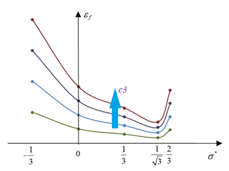
    Using this method, it is easy to change the failure curve by adjusting the single plastic failure strain in uniaxial tension value, c3.


    Figure 3. Changes in Plastic Failure Strain Curve. by increasing the uniaxial tension failure, c3, with the same failure plastic strain ratios

Default Behavior

By default, the values different than 0 for c1 to c5 need to be entered. However, specific default behaviors exists, in case failure information are missing.
  • In case the material failure behavior is unknown, c1 to c5 are set to 0.0 and the mild steel behavior (M-Flag=1) is used.
  • If only the tensile failure value is known, c3 is defined ( c 1 = c 2 = c 4 = c 5 = 0.0 MathType@MTEF@5@5@+= feaagKart1ev2aaatCvAUfeBSjuyZL2yd9gzLbvyNv2CaerbuLwBLn hiov2DGi1BTfMBaeXatLxBI9gBaerbd9wDYLwzYbItLDharqqtubsr 4rNCHbGeaGqiVu0Je9sqqrpepC0xbbL8F4rqqrFfpeea0xe9Lq=Jc9 vqaqpepm0xbba9pwe9Q8fs0=yqaqpepae9pg0FirpepeKkFr0xfr=x fr=xb9adbaqaaeGaciGaaiaabeqaamaabaabaaGcbaGaam4yaiaaig dacqGH9aqpcaWGJbGaaGOmaiabg2da9iaadogacaaI0aGaeyypa0Ja am4yaiaaiwdacqGH9aqpcaaIWaGaaiOlaiaaicdaaaa@42C8@ ). The mild steel behavior is used and scaled by the user- defined c3 value.
  • In case the material behavior is known, M-Flag is defined and c3 can be used to adjust the failure model according the expected tensile failure. The selected material behavior is scaled by the user-defined c3 value.
  • For all other cases, all c1 to c5 are intended to be defined and default value of 0.0 is used.

Element Failure Treatment

A cumulative damage method is used to sum the amount of plastic strain that has occurred at each integration point in the element using:(3)
D= Δ ε p ε f 1 MathType@MTEF@5@5@+= feaagKart1ev2aqatCvAUfeBSjuyZL2yd9gzLbvyNv2CaerbuLwBLn hiov2DGi1BTfMBaeXatLxBI9gBaerbd9wDYLwzYbItLDharqqtubsr 4rNCHbGeaGqiVu0Je9sqqrpepC0xbbL8F4rqqrFfpeea0xe9Lq=Jc9 vqaqpepm0xbba9pwe9Q8fs0=yqaqpepae9pg0FirpepeKkFr0xfr=x fr=xb9adbaqaaeGaciGaaiaabeqaamaabaabaaGcbaGaamiraiabg2 da9maaqaeabaWaaSaaaeaacaqGuoGaeqyTdu2aaSbaaSqaaiaadcha aeqaaaGcbaGaeqyTdu2aaSbaaSqaaiaadAgaaeqaaaaakiabgwMiZk aaigdaaSqabeqaniabggHiLdaaaa@431F@
Where,
D MathType@MTEF@5@5@+= feaagKart1ev2aaatCvAUfeBSjuyZL2yd9gzLbvyNv2CaerbuLwBLn hiov2DGi1BTfMBaeXatLxBI9gBaerbd9wDYLwzYbItLDharqqtubsr 4rNCHbGeaGqiVu0Je9sqqrpepC0xbbL8F4rqqrFfpeea0xe9Lq=Jc9 vqaqpepm0xbba9pwe9Q8fs0=yqaqpepae9pg0FirpepeKkFr0xfr=x fr=xb9adbaqaaeGaciGaaiaabeqaamaabaabaaGcbaGaamiraaaa@36BF@
Damage
Δ ε p MathType@MTEF@5@5@+= feaagKart1ev2aaatCvAUfeBSjuyZL2yd9gzLbvyNv2CaerbuLwBLn hiov2DGi1BTfMBaeXatLxBI9gBaerbd9wDYLwzYbItLDharqqtubsr 4rNCHbGeaGqiVu0Je9sqqrpepC0xbbL8F4rqqrFfpeea0xe9Lq=Jc9 vqaqpepm0xbbG8FasPYRqj0=yi0dXdbba9pGe9xq=JbbG8A8frFve9 Fve9Ff0dmeaabaqaciGacaGaaeqabaWaaeaaeaaakeaacaqGuoGaeq yTdu2aaSbaaSqaaiaadchaaeqaaaaa@3A40@
The change in plastic strain of the integration point
ε f MathType@MTEF@5@5@+= feaagKart1ev2aqatCvAUfeBSjuyZL2yd9gzLbvyNv2CaerbuLwBLn hiov2DGi1BTfMBaeXatLxBI9gBaerbd9wDYLwzYbItLDharqqtubsr 4rNCHbGeaGqiVu0Je9sqqrpepC0xbbL8F4rqGqFfpeea0xe9vq=Jb9 vqpeea0xd9q8qiYRWxGi6xij=hbba9q8aq0=yq=He9q8qiLsFr0=vr 0=vr0db8meaabaqaciGacaGaaeqabaWaaeaaeaaakeaacqaH1oqzda WgaaWcbaGaamOzaaqabaaaaa@3A26@
Plastic failure strain for the current stress triaxiality

In shell elements after an integration point reaches D = 1 MathType@MTEF@5@5@+= feaagKart1ev2aqatCvAUfeBSjuyZL2yd9gzLbvyNv2CaerbuLwBLn hiov2DGi1BTfMBaeXatLxBI9gBaerbd9wDYLwzYbItLDharqqtubsr 4rNCHbGeaGqiVu0Je9sqqrpepC0xbbL8F4rqqrFfpeea0xe9Lq=Jc9 vqaqpepm0xbbG8FasPYRqj0=yi0dXdbba9pGe9xq=JbbG8A8frFve9 Fve9Ff0dmeaabaqaciGacaGaaeqabaWaaeaaeaaakeaacaWGebGaey ypa0JaaGymaaaa@38E9@ , the integration point’s stress tensor is set to zero. The element fails and is deleted when the percentage of through thickness failed integration points equals P_thickfail. In solid elements, the element is deleted when any integration point reaches D = 1 MathType@MTEF@5@5@+= feaagKart1ev2aqatCvAUfeBSjuyZL2yd9gzLbvyNv2CaerbuLwBLn hiov2DGi1BTfMBaeXatLxBI9gBaerbd9wDYLwzYbItLDharqqtubsr 4rNCHbGeaGqiVu0Je9sqqrpepC0xbbL8F4rqqrFfpeea0xe9Lq=Jc9 vqaqpepm0xbbG8FasPYRqj0=yi0dXdbba9pGe9xq=JbbG8A8frFve9 Fve9Ff0dmeaabaqaciGacaGaaeqabaWaaeaaeaaakeaacaWGebGaey ypa0JaaGymaaaa@38E9@ .

Plane Strain as Global Minimum

The S-Flag=2 option can be used to force the global minimum of the plastic failure strain curve to occur at the plane strain stress triaxiality location, c4. This is accomplished by splitting the second equation into 2 separate quadratic sub-functions.

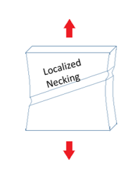
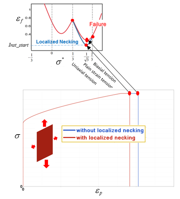
Modeling Material Instability (Localized Necking)

In materials such as sheet metal, thickness thinning and diffuse necking may appear during tensile loading of the material. This is called localized necking and normally occurs in the stress triaxiality range of 1 3 σ * 2 3 MathType@MTEF@5@5@+= feaagKart1ev2aqatCvAUfeBSjuyZL2yd9gzLbvyNv2CaerbuLwBLn hiov2DGi1BTfMBaeXatLxBI9gBaerbd9wDYLwzYbItLDharqqtubsr 4rNCHbGeaGqiVCI8FfYJH8YrFfeuY=Hhbbf9v8qqaqFr0xc9pk0xbb a9q8WqFfeaY=biLkVcLq=JHqpepeea0=as0Fb9pgeaYRXxe9vr0=vr 0=vqpWqaaeaabiGaciaacaqabeaadaqaaqaaaOqaamaalaaabaGaaG ymaaqaaiaaiodaaaaeaaaaaaaaa8qacqGHKjYOcqaHdpWCpaWaaWba aSqabeaapeGaaiOkaaaak8aacqGHKjYOdaWcaaqaaiaaikdaaeaaca aIZaaaaaaa@3F5D@ :


Figure 4.
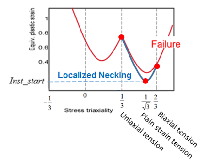
In /FAIL/BIQUAD it is possible to simulate this localized necking using the option, S-Flag=3 and Inst_start. This option uses the same plastic failure strain curve as S-Flag=2 and adds two additional quadratic functions that define a curve that represents the start of localized necking between stress triaxiality 1 3 MathType@MTEF@5@5@+= feaagKart1ev2aqatCvAUfeBSjuyZL2yd9gzLbvyNv2CaerbuLwBLn hiov2DGi1BTfMBaeXatLxBI9gBaerbd9wDYLwzYbItLDharqqtubsr 4rNCHbGeaGqiVCI8FfYJH8YrFfeuY=Hhbbf9v8qqaqFr0xc9pk0xbb a9q8WqFfeaY=biLkVcLq=JHqpepeea0=as0Fb9pgeaYRXxe9vr0=vr 0=vqpWqaaeaabiGaciaacaqabeaadaqaaqaaaOqaamaalaaabaGaaG ymaaqaaiaaiodaaaaaaa@3774@ and 2 3 MathType@MTEF@5@5@+= feaagKart1ev2aqatCvAUfeBSjuyZL2yd9gzLbvyNv2CaerbuLwBLn hiov2DGi1BTfMBaeXatLxBI9gBaerbd9wDYLwzYbItLDharqqtubsr 4rNCHbGeaGqiVCI8FfYJH8YrFfeuY=Hhbbf9v8qqaqFr0xc9pk0xbb a9q8WqFfeaY=biLkVcLq=JHqpepeea0=as0Fb9pgeaYRXxe9vr0=vr 0=vqpWqaaeaabiGaciaacaqabeaadaqaaqaaaOqaamaalaaabaGaaG ymaaqaaiaaiodaaaaaaa@3774@ . The minimum value of this curve is a user-defined value in the Inst_start field and occurs at plane strain tension σ * = 1 3 MathType@MTEF@5@5@+= feaagKart1ev2aqatCvAUfeBSjuyZL2yd9gzLbvyNv2CaerbuLwBLn hiov2DGi1BTfMBaeXatLxBI9gBaerbd9wDYLwzYbItLDharqqtubsr 4rNCHbGeaGqiVCI8FfYJH8YrFfeuY=Hhbbf9v8qqaqFr0xc9pk0xbb a9q8WqFfeaY=biLkVcLq=JHqpepeea0=as0Fb9pgeaYRXxe9vr0=vr 0=vqpWqaaeaabiGaciaacaqabeaadaqaaqaaaOqaaabaaaaaaaaape Gaeq4Wdm3damaaCaaaleqabaWdbiaacQcaaaGcpaGaeyypa0ZaaSaa aeaacaaIXaaabaWaaOaaaeaacaaIZaaaleqaaaaaaaa@3B8B@ . Using this localized necking curve, a second localized necking damage value is calculated and failure due to necking only occurs when all integration points reach D = 1 MathType@MTEF@5@5@+= feaagKart1ev2aqatCvAUfeBSjuyZL2yd9gzLbvyNv2CaerbuLwBLn hiov2DGi1BTfMBaeXatLxBI9gBaerbd9wDYLwzYbItLDharqqtubsr 4rNCHbGeaGqiVu0Je9sqqrpepC0xbbL8F4rqqrFfpeea0xe9Lq=Jc9 vqaqpepm0xbbG8FasPYRqj0=yi0dXdbba9pGe9xq=JbbG8A8frFve9 Fve9Ff0dmeaabaqaciGacaGaaeqabaWaaeaaeaaakeaacaWGebGaey ypa0JaaGymaaaa@38E9@ . The localized necking criteria is based on the Marciniak-Kuczynski analysis. 1


Figure 5. Default Failure Strain Curve . with additional localized necking curve (blue)

When using S-Flag=1 or 2, the damage accumulation begins once the plastic strain reaches in failure curve (red in Figure 6).

If S-Flag=3is used to describe the localized necking, damage accumulation begins once the plastic strain reaches in the localized necking curve (blue curve in Figure 6). For localized necking, the element is deleted when all integration points reach damage, D = 1 MathType@MTEF@5@5@+= feaagKart1ev2aqatCvAUfeBSjuyZL2yd9gzLbvyNv2CaerbuLwBLn hiov2DGi1BTfMBaeXatLxBI9gBaerbd9wDYLwzYbItLDharqqtubsr 4rNCHbGeaGqiVu0Je9sqqrpepC0xbbL8F4rqqrFfpeea0xe9Lq=Jc9 vqaqpepm0xbbG8FasPYRqj0=yi0dXdbba9pGe9xq=JbbG8A8frFve9 Fve9Ff0dmeaabaqaciGacaGaaeqabaWaaeaaeaaakeaacaWGebGaey ypa0JaaGymaaaa@38E9@ , whereas element deletion not due to localized necking is defined by P_thickfail.


Figure 6.

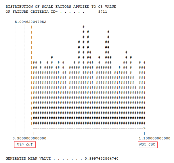
Perturbation of the Failure Limit

Due to a materials imperfection or production process, a material’s failure strain may not be exactly the same everywhere and thus very small perturbations of failure limit may exist. When using M-Flag>0 with /PERTURB/FAIL/BIQUAD, a statistical distribution of the failure limit is applied to each element assigned the failure model. This is accomplished by calculating the normal or random distribution of a failure scale factor which is applied to /FAIL/BIQUAD, c3. 
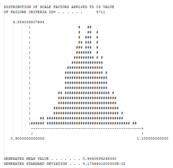
The two different distributions methods are shown in Figure 7 and Figure 8.


Figure 7. Random Distribution. Idistri=1, of the failure limit in the Starter *0.out file


Figure 8. Normal (Gaussian) Distribution. Idistri=2, of the failure limit in the Starter *0.out file
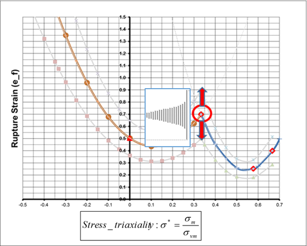
/FAIL/BQUAD uses small perturbations of c3 generated by /PERTURB/FAIL/BIQUAD to scale the entire failure curve using the strain ratio values for the predefined materials or user-defined ratios, r1, r2, r4 and r5, depending on the value of M-Flag.


Figure 9.

Reference

1 Pack, Keunhwan, and Dirk Mohr. "Combined necking & fracture model to predict ductile failure with shell finite elements." Engineering Fracture Mechanics 182 (2017): 32-51