Right-click at the Report or Chapter level and select Add > Items > Image.
Or
From the Report Ribbon, Add Item tool group,
click Image.Figure 1.
.
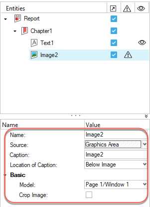
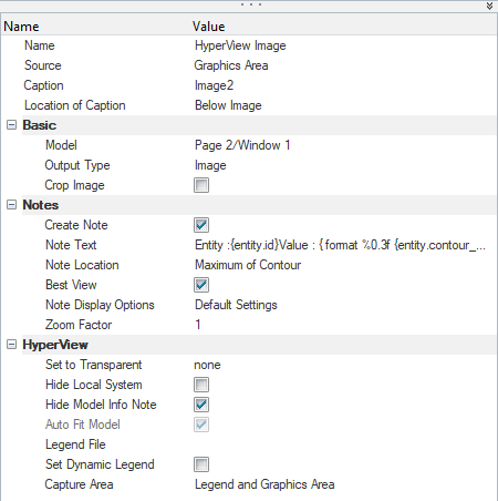
Below are the properties associated with the Image entity.
Note: Image properties are HyperWorks client
dependent. They are listed below.
HyperMesh properties Figure 2.
Name: You can change the name property of the image
item.
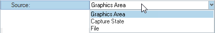
Source: Select the image source. Figure 3.
Graphics Area: Capture an image from the graphics
area.
Capture State: Enables you to capture an image using
a dynamic rectangle. If selected, the
Capture Dynamic Rectangle
option is activated. Check this option and capture
the image by drawing a rectangle anywhere in the
screen.
Caption: Provide a caption for the captured image. This
caption is visible in the exported Document report.
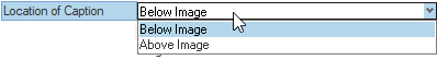
Location of Caption: Select the caption location from the
list. These are standard locations as present in Microsoft
Word. Image captions locations can be:
Below Image, or
Above Image Figure 4.
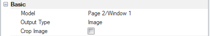
Basic
Model: Select the required page or window from the HyperWorks session.
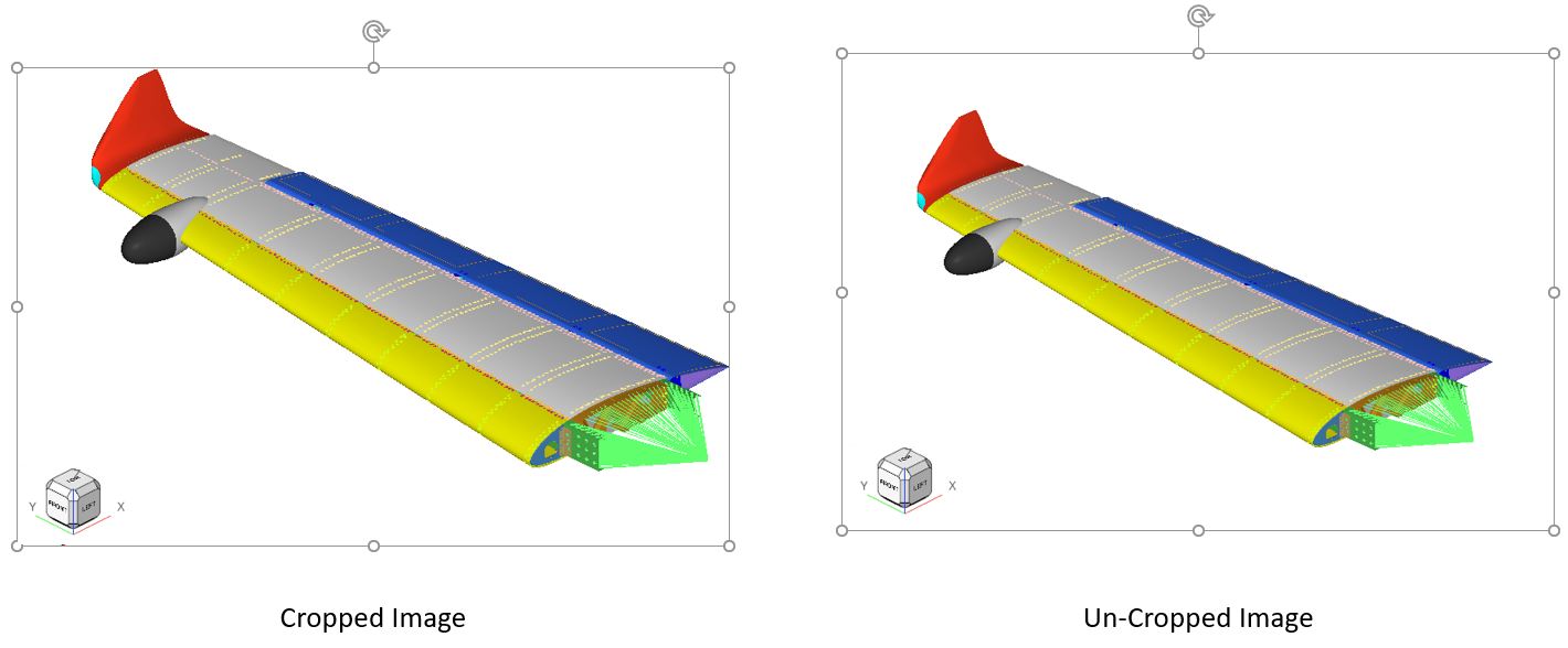
Crop Image: Checkbox option to crop an image. This option
discards empty/white space in the graphics area and exports
only the model area. Below is an illustration of the crop
image option. Figure 5.
HyperView properties Figure 6.
The first four properties are the same as the HyperMesh client.
Basic
Model: Select the required page or window from the HyperWorks session.
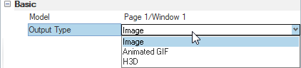
Output Type: Choose between various output formats for the
exported image. The available output types are: Figure 7.
Image: A .png (static) image is
exported.
Animated GIF: A standard animation file is exported.
The GIF option is supported only for Presentation
reports.
H3D: A HyperView results
file with the animation is exported.
Note: H3D
preview is not available on LibreOffice
5.0.
Crop Image: Checkbox option to crop an image.
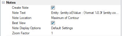
Notes Figure 8.
Create Note: Checkbox option to create notes in the images.
This activates other note creation options.
Note Text: Enter the desired query options in the
Define Text dialog.
Note:
You can manually enter the expressions or query
statements. The same syntax from the Description
section of the Note creation panel in HyperView can be followed.
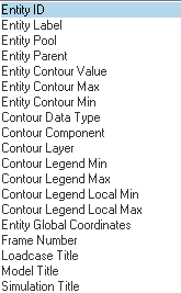
You can also configure note expressions using
the array of default note query options. Select a
note type and click Insert.
This query is added to the note and will be
exported to an image in the report. The list is
shown below. Figure 9.
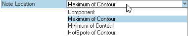
Note Location: Select the location for the notes to be
created. Supported note locations are: Figure 10.
Component: Notes are created at the CoG of the
component.
Maximum of Contour: Notes are created where the
maximum contour value is seen in an entity.
Minimum of Contour: Notes are created where the
minimum contour value is seen in an entity.
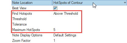
Hotspots of Contour: Notes are created at hotspots
of an entity. There are a few options that are
required to capture the hotspot values. They are
listed below. Figure 11.
Find Hotspots: Find hotspots for values above
or below threshold values.
Threshold: Numerical value to define the
threshold.
Tolerance: Numerical value to define the
tolerance between contour values of two adjacent
elements.
Maximum Hotspots: Number for hotspots for note creation.
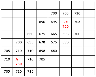
Note:
The hotspot detection algorithm first finds
the element with the highest contour value (center
element). It then finds the adjacent elements and
their contour values. If these contour values are
lower than the center element, then the elements
adjacent to these elements are found and
correspondingly the contour values. This is
repeated until an element is found that has a
contour value higher than its center element by
the Tolerance specified by you. This element is
considered as the new hotspot.
For example, if you have set the tolerance as
50, element A has the highest contour values
(750). ARD finds adjacent elements and their
contour values (710, 670, 665) until it finds the
element B (710) which has the highest value. B
shows 720 in the image. Figure 12.
Best View: When enabled, this option sets the best view
possible for the entity and captures the image.
The Best View algorithm finds the element at which
the maximum/minimum contour value is seen.
Then, it finds the element normal direction at this
critical element and accordingly sets the view of
the model to be captured in the image.
Note Display Options: You can select the style for the notes
from the list. Any custom note styles present in the
selected Model page are listed.
Zoom factor: Set the magnification value from zero to ten.
This specified zoom factor is applied to that entity where
the Note is created.
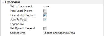
HyperView Settings
Figure 13.
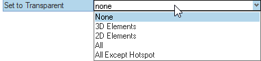
Set to Transparent: You can define the transparency settings
for the entities in the model. The supported transparency
options are: Figure 14.
None - None of the elements are set to
transparent.
3D Elements - Only 3D elements are set to
transparent.
2D Elements - Only 2D elements are set to
transparent.
All - All of the elements are set to
transparent.
All Except Hotspot - Except for the component or
group on which maximum/minimum/hotspots are seen,
all others are set to transparent.
Hide Local Systems: Select this checkbox to hide all of the
local coordinate systems from being included in the report
images.
Hide Model Info Note: Select this checkbox to hide the model
information note from the report images.
Auto Fit Model: Select this option to auto fit the model. If
the Best View option is selected, then Auto Fit is
automatically applied to the model.
Note: If Best View is
enabled, the auto fit is applied to the model even
though the Auto Fit option is not enabled. Hence, when
you select the Best View option, the Auto Fit option is
disabled in the panel.
Legend File: Specify the legend file to be used to update
the contour legend. A file selection option is enabled once
the box is checked.
Set Dynamic Legend: Specify if the legend type is to be set
to the Dynamic scale. If selected, the legend of the contour
is automatically updated for only Displayed entities. This
option is helpful when an image is looped over some result
type and if the legend of the contour is to be dynamically
updated for each displayed component considered under
looping
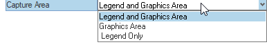
Capture Area: Select the image capture area. Figure 15.
Legend and Graphic Area: The Legend and Graphics
area are both captured.
Graphics Area: Only the graphics area is
captured.
Legend Only: Only the contour legend is
captured
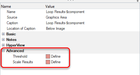
Advanced Options
When an image entity is added under a
Loop Results module, additional results processing properties
are activated. They are listed below. Figure 16.
To utilize the advanced options, you have to select
components and loadcases for the Loop Results module
first.
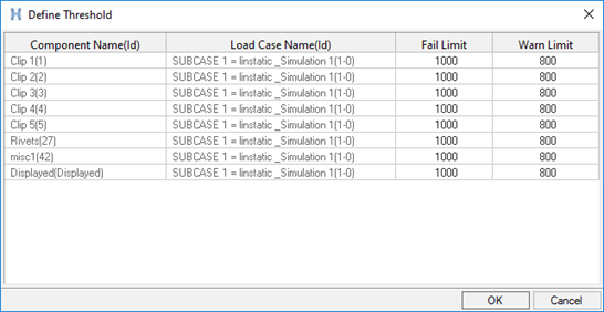
Threshold: Define the Fail and Warn limits for the results
looping.
Fail and Warn limits are suggested
automatically based on the contour values of the applied
results. You can edit them as well. Figure 17.
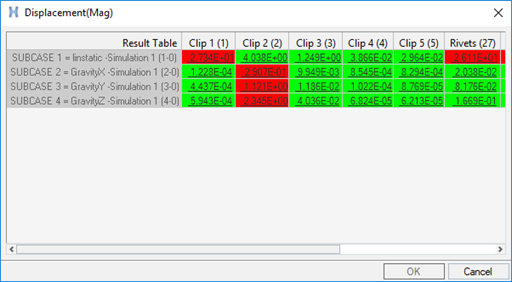
Once executed, a results table with the
color codes is added to the report.
Red for Fail
Yellow for Warn
Green for Safe
Figure 18.
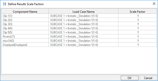
Scale: Scale contour results for looping. Figure 19.
Scale factor is set to one by default; you can edit
them as well.
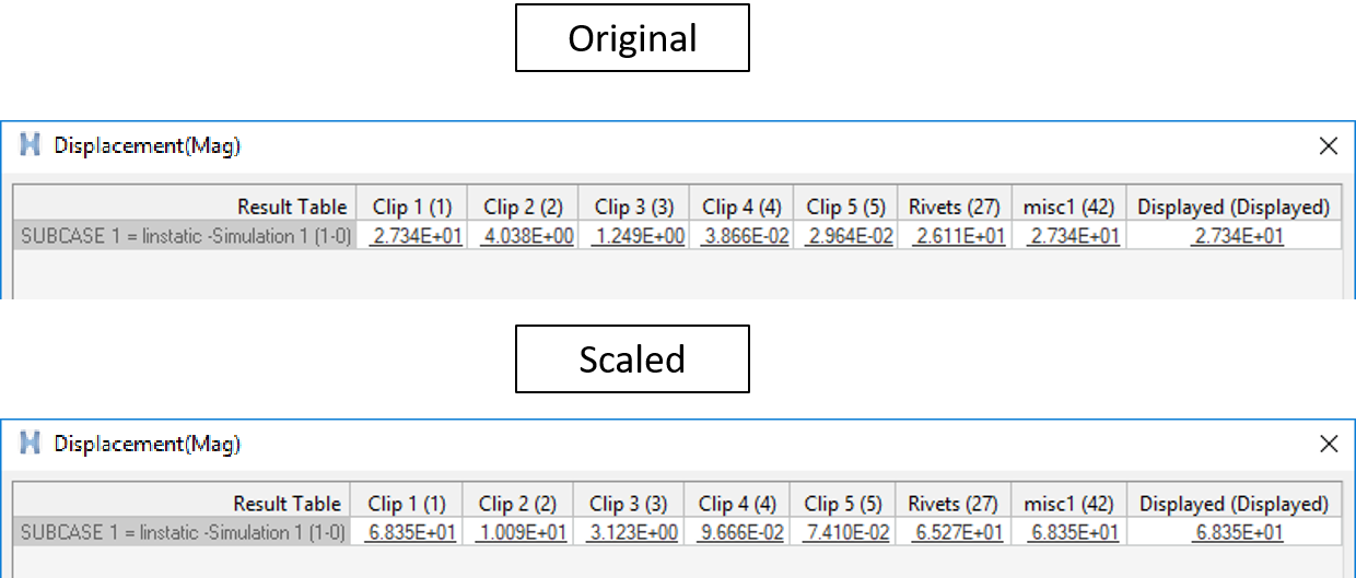
Once executed, a result table with
the scaled results with the scale factor is added to the
report. Figure 20.
 Figure 1.