HS-1615: Set Up a FEKO Model
Learn how to set up a FEKO model in HyperStudy.
Before you begin, copy the model files used in
this tutorial from <hst.zip>/HS-1615/ to your working
directory.
The model used in this tutorial is a waveguide transmission line that is being fed with a coaxial cable.
The effect of the cable’s pin position on input impedence is studied. When the impedence is reduced, this leads to improved power transmission.
Perform the Study Setup
-
Start a new study in the following ways:
- From the menu bar, click .
- On the ribbon, click
 .
.
-
Add a FEKO model by dragging-and-dropping the
waveguide_pin_feed_placement.cfx from the Directory
into the work area.
The Resource, Solver input file, and Solver input arguments fields become populated.
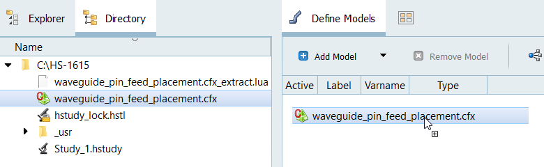
Figure 1. -
Review the input variables.
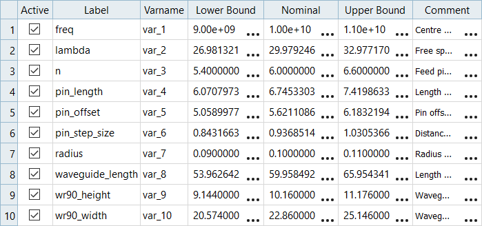
Figure 2.
Perform Nominal Run
Create and Evaluate Output Responses
In this step you will create two output responses.
-
Create output response 1.
-
Define the following and click Next.
- Set Type to Output.
- Set Request to z_Imag.
- Set Component to Value.
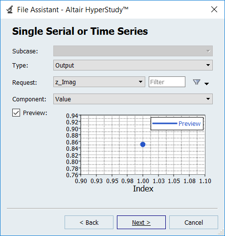
Figure 3. -
Click Finish.
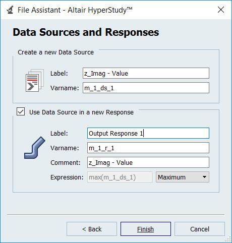
Figure 4.
Output response 1 is added to the work area. -
Define the following and click Next.
Run DOE
-
In the Settings tab, change the Number of runs to
21.
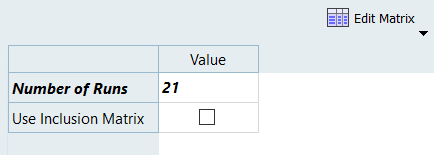
Figure 5.
Run Fit
-
Import matrix.
- Click Add Matrix.
- In the Matrix Source column, select DOE 1 (doe_1).
- Click Import Matrix.

Figure 6. -
In the work area, Fit Type column, select Radial Basis
Function for both output responses.
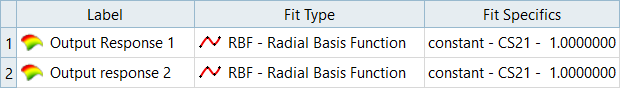
Figure 7. -
Plot the response surface.
- Click the Trade-Off tab.
- Using the Channel selector, select both output responses.
- From the Inputs section, select the X Axis checkbox.
-
From the Output Plots section, select
 (Multiplot).
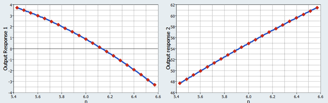
Figure 8.