Two-Phase Nucleate Boiling in a Cylindrical Pipe
In this application, AcuSolve is used to simulate the changes in wall temperature due to two-phase nucleate boiling at the heated walls of a pipe with water flowing through it. AcuSolve results are compared with experimental results adapted from Koncar and others (2015). The close agreement of AcuSolve results with experimental results validates the ability of AcuSolve to model two-phase nucleate boiling problems.
Problem Description
The problem consists of a pipe with heated surrounding walls, as shown in the following image, which is not drawn to scale. The length of the pipe is 2 m and the radius is 0.0017 m. Mass flux at the inlet is 900 kg/m2 and the temperature of the fluid entering the pipe is 473 K. A heat flux of 570,000 W/m2 is applied on the walls. The preheated water enters the inlet and heat is transferred to the fluid from the walls. The heat causes sub-cooled boiling to occur in the region close to the wall and leads to the formation of bubbles at nucleation sites.
During sub-cooled boiling flow, heat and mass exchange between the phases takes place on the heated wall and in sub-cooled liquid flow. On the heated surface the vapor bubbles are generated and as they move through the sub-cooled liquid they condense and release the latent heat.
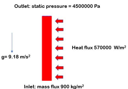
Figure 1. Parameters for Simulating a Two-Phase Nucleate Boiling Problem of a Pipe
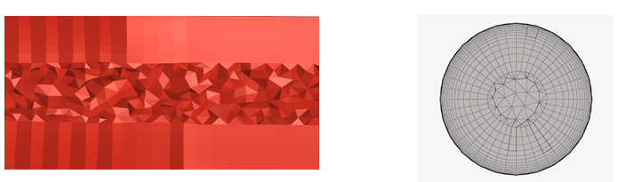
Figure 2. Mesh used for Simulating Two-Phase Flow in a Pipe
AcuSolve Results
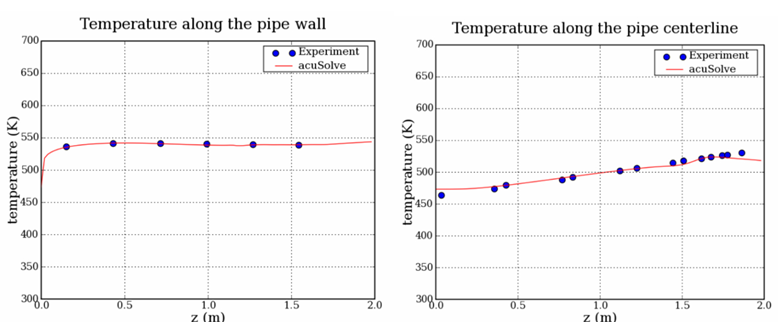
Figure 3. Temperature Values for Varying Streamwise Distance Compared to Experimental Data
Summary
The AcuSolve solution compares well with experimental results for two-phase nucleate boiling simulations. In this application, the temperature of the wall as the onset of boiling approaches are simulated with AcuSolve using the nucleate boiling feature and the SA turbulence model. The experimental values of temperature are presented with the corresponding AcuSolve results. A good agreement of simulation results with the experiment validates the ability to solve two-phase nucleate boiling using the nucleate boiling capabilities of AcuSolve.
Simulation Settings for Two-Phase Nucleate Boiling in a Cylindrical Pipe
HyperWorks database file: <your working directory>\pipe_two_phase_boiling\pipe_two_phase_boiling.hm.
Global
- Problem Description
- Analysis type – Transient
- Turbulence equation – SA
- Temperature equation – Advective Diffusive
- Auto Solution Strategy
- Maximum time steps – 500
- Initial time increment – 0.003
- Convergence Tolerance – 0.001 sec
- Relaxation factor – 0.3
- Surface Tension Model (“Water_NB-Vapor_NB”)
- Type – Constant
- Surface Tension – 0.02382
- Material Model
- Vapor_NB
- Type – Constant
- Density – 23.75 kg/m3
- Viscosity – 1.79e-05 kg/m-sec
- Specific Heat – 4225 J/kg-K
- Latent Heat – 1675570
- Latent Heat Temperature – 530.55 K
- Conductivity – 0.02528 W/m-K
- Water_NB
- Type – Constant
- Density – 800 kg/m3
- Viscosity – 0.0001339 kg/m-sec
- Specific Heat – 4500 J/kg-K
- Conductivity – 0.65 W/m-K
- Vapor_NB
- Multifield parameter (Field interaction model)
- Type – Algebraic Eulerian
- Phase change type – Wall Boiling
- Carrier field - Water
- Disperse field – Vapor
- Disperse field diameter type – Boiling kurul exponential
- Drag model – Ishii zuber
- Lift Model – Legendre Magnaudet
Model
- Volumes
- Fluid
- Material – Vapor_Water
- Fluid
- Surfaces
- Inflow
- Simple Boundary Condition – Inflow
- Inflow type – Mass Flux Rate
- Mass Flux Rate – 0.167634 kg/sec
- Temperature – 473 K
- Outflow
- Simple Boundary Condition – Outflow
- Pressure – 4500000 N/m2
- Wall
- Simple Boundary Condition – Wall
- Temperature type – Flux
- Heat Flux – 570000 W/m2
- Inflow
References
B. Koncar, E. Krapper, Y. Egorov, 2005, “CFD MODELING OF SUBCOOLED FLOW BOILING FOR NUCLEAR ENGINEERING APPLICATIONS”, International Conference Nuclear Energy for New Europe 2005, Bled, Slovenia, September 5-8,2005.