AI Card
This card defines an impressed current source that varies linearly between the values at the start and end points.
On the Source/Load tab, in the Ideal sources
group, click the ![]() Impressed current
icon. From the drop-down list, click the
Impressed current
icon. From the drop-down list, click the ![]() Impressed current in space (AI) icon.
Impressed current in space (AI) icon.
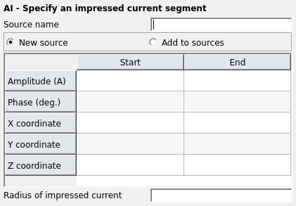
Figure 1. The AI - Specify an impressed current segment dialog.

Figure 2. Impressed line current with a linear current distribution.
Parameters:
- New source
- A new excitation is defined which replaces all previously defined excitations.
- Add to sources
- A new excitation is defined which is added to the previously defined excitations.
- Amplitude (A)
- Amplitude |I1| in A of the current at the start point, r1, and end point, r2.
- Phase (deg.)
- Phase of the current at the start and end points in degrees.
- X, Y, Z coordinate
- Coordinates of the start and end points in m. (Note that all the coordinate values are optionally scaled by the SF card.)
- Radius of impressed current
- This parameter is optional. If specified, and different from zero, this value gives a finite wire radius for the impressed current element. Feko then assumes that the current is uniformly distributed on the wire surface and uses the exact wire integral. If this parameter is not specified, the current filament approximation is used. (This value is optionally scaled by the SF card.)
The following restrictions apply when using the impressed current elements:
- It is not possible to attach the impressed current to a wire segment. (If the impressed current is making electrical contact with a triangular surface current element, the AV card should be used.)
- When modelling dielectric bodies with the surface equivalence principle, the current element must be in the free space medium, that is outside the dielectric bodies. (The material parameters of this medium can, however, be set with the EG and/or GF cards).
- When used with the spherical Green’s function, the current element must be outside the dielectric spheres.
- The current segments may be joined with each other and with the AV card to form long paths and/or closed loops. The point charges that arise when the current does not go to zero at an end point or when there is a current discontinuity at a connection point, are not taken into consideration. This is required to model, for example, the case where radiating lines are terminated in a non-radiating structure. If these charges must be considered explicitly, the line current should be modelled by a row of Hertzian dipoles (see the A5 card). Note, however, that the constant line charge along the current segment is correctly taken into account.
- If several of these current elements are used, the total radiated power (required to calculate, for example, the far field gain/directivity) can only be calculated accurately if the mutual coupling between segments is taken into account. Due to neglecting the point charges at the ends of the segments, the coupling cannot be determined accurately. If exact values of the radiated power are required, it should be determined by integrating the far field (see the FF card). It should be noted that, for example, the computed near and far fields (the actual field strength values), the induced currents, coupling factors and losses are computed correctly.