SPH Cell Distribution

It is recommended to distribute the particles through a hexagonal compact or a cubic net.

Hexagonal Compact Net

A cubic centered faces net realizes a hexagonal compact distribution and this can be useful to build the net (Figure 1). The nominal value h 0 MathType@MTEF@5@5@+= feaagKart1ev2aaatCvAUfeBSjuyZL2yd9gzLbvyNv2CaerbuLwBLn hiov2DGi1BTfMBaeXatLxBI9gBaerbd9wDYLwzYbItLDharqqtubsr 4rNCHbGeaGqiVu0Je9sqqrpepC0xbbL8F4rqqrFfpeea0xe9Lq=Jc9 vqaqpepm0xbba9pwe9Q8fs0=yqaqpepae9pg0FirpepeKkFr0xfr=x fr=xb9adbaqaaeGaciGaaiaabeqaamaabaabaaGcbaGaamiAamaaBa aaleaacaaIWaaabeaaaaa@37C9@ is the distance between any particle and its closest neighbor. The mass of the particle m p MathType@MTEF@5@5@+= feaagKart1ev2aaatCvAUfeBSjuyZL2yd9gzLbvyNv2CaerbuLwBLn hiov2DGi1BTfMBaeXatLxBI9gBaerbd9wDYLwzYbItLDharqqtubsr 4rNCHbGeaGqiVu0Je9sqqrpepC0xbbL8F4rqqrFfpeea0xe9Lq=Jc9 vqaqpepm0xbba9pwe9Q8fs0=yqaqpepae9pg0FirpepeKkFr0xfr=x fr=xb9adbaqaaeGaciGaaiaabeqaamaabaabaaGcbaGaamyBamaaBa aaleaacaWGWbaabeaaaaa@3809@ may be related to the density of the material ρ and to the size h 0 MathType@MTEF@5@5@+= feaagKart1ev2aaatCvAUfeBSjuyZL2yd9gzLbvyNv2CaerbuLwBLn hiov2DGi1BTfMBaeXatLxBI9gBaerbd9wDYLwzYbItLDharqqtubsr 4rNCHbGeaGqiVu0Je9sqqrpepC0xbbL8F4rqqrFfpeea0xe9Lq=Jc9 vqaqpepm0xbba9pwe9Q8fs0=yqaqpepae9pg0FirpepeKkFr0xfr=x fr=xb9adbaqaaeGaciGaaiaabeqaamaabaabaaGcbaGaamiAamaaBa aaleaacaaIWaaabeaaaaa@37C9@ of the hexagonal compact net, with respect to:(1)
m p h 0 3 2 ρ
Since the space can be partitioned into polyhedras surrounding each particle of the net, each one with a volume:(2)
V p h 0 3 2

But, due to discretization error at the frontiers of the domain, mass consistency better corresponds to m P = ρ V n .

Where,
V MathType@MTEF@5@5@+= feaagKart1ev2aaatCvAUfeBSjuyZL2yd9gzLbvyNv2CaerbuLwBLn hiov2DGi1BTfMBaeXatLxBI9gBaerbd9wDYLwzYbItLDharqqtubsr 4rNCHbGeaGqiVu0Je9sqqrpepC0xbbL8F4rqqrFfpeea0xe9Lq=Jc9 vqaqpepm0xbba9pwe9Q8fs0=yqaqpepae9pg0FirpepeKkFr0xfr=x fr=xb9adbaqaaeGaciGaaiaabeqaamaabaabaaGcbaGaamOvaaaa@36D1@
Total volume of the domain and n MathType@MTEF@5@5@+= feaagKart1ev2aaatCvAUfeBSjuyZL2yd9gzLbvyNv2CaerbuLwBLn hiov2DGi1BTfMBaeXatLxBI9gBaerbd9wDYLwzYbItLDharqqtubsr 4rNCHbGeaGqiVu0Je9sqqrpepC0xbbL8F4rqqrFfpeea0xe9Lq=Jc9 vqaqpepm0xbba9pwe9Q8fs0=yqaqpepae9pg0FirpepeKkFr0xfr=x fr=xb9adbaqaaeGaciGaaiaabeqaamaabaabaaGcbaGaamOBaaaa@36E9@ the number of particles distributed in the domain
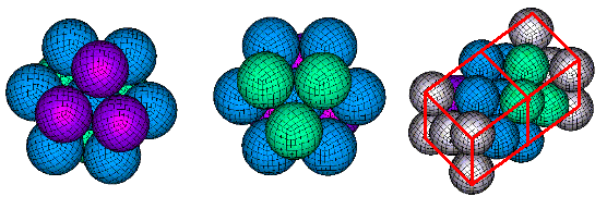
Figure 1. Local View of Hexagonal Compact Net and Perspective View of Cubic Centered Faces Net
Note: Choosing h 0 MathType@MTEF@5@5@+= feaagKart1ev2aaatCvAUfeBSjuyZL2yd9gzLbvyNv2CaerbuLwBLn hiov2DGi1BTfMBaeXatLxBI9gBaerbd9wDYLwzYbItLDharqqtubsr 4rNCHbGeaGqiVu0Je9sqqrpepC0xbbL8F4rqqrFfpeea0xe9Lq=Jc9 vqaqpepm0xbba9pwe9Q8fs0=yqaqpepae9pg0FirpepeKkFr0xfr=x fr=xb9adbaqaaeGaciGaaiaabeqaamaabaabaaGcbaGaamiAamaaBa aaleaacaaIWaaabeaaaaa@37C9@ for the smoothing length insures naturally consistency up to order 1 if the previous equation is satisfied.

Weight functions vanish at distance 2 h MathType@MTEF@5@5@+= feaagKart1ev2aaatCvAUfeBSjuyZL2yd9gzLbvyNv2CaerbuLwBLn hiov2DGi1BTfMBaeXatLxBI9gBaerbd9wDYLwzYbItLDharqqtubsr 4rNCHbGeaGqiVu0Je9sqqrpepC0xbbL8F4rqqrFfpeea0xe9Lq=Jc9 vqaqpepm0xbba9pwe9Q8fs0=yqaqpepae9pg0FirpepeKkFr0xfr=x fr=xb9adbaqaaeGaciGaaiaabeqaamaabaabaaGcbaGaaGOmaiaadI gaaaa@379F@ where h MathType@MTEF@5@5@+= feaagKart1ev2aaatCvAUfeBSjuyZL2yd9gzLbvyNv2CaerbuLwBLn hiov2DGi1BTfMBaeXatLxBI9gBaerbd9wDYLwzYbItLDharqqtubsr 4rNCHbGeaGqiVu0Je9sqqrpepC0xbbL8F4rqqrFfpeea0xe9Lq=Jc9 vqaqpepm0xbba9pwe9Q8fs0=yqaqpepae9pg0FirpepeKkFr0xfr=x fr=xb9adbaqaaeGaciGaaiaabeqaamaabaabaaGcbaGaaGOmaiaadI gaaaa@379F@ is the smoothing length. In an hexagonal compact net with size h 0 MathType@MTEF@5@5@+= feaagKart1ev2aaatCvAUfeBSjuyZL2yd9gzLbvyNv2CaerbuLwBLn hiov2DGi1BTfMBaeXatLxBI9gBaerbd9wDYLwzYbItLDharqqtubsr 4rNCHbGeaGqiVu0Je9sqqrpepC0xbbL8F4rqqrFfpeea0xe9Lq=Jc9 vqaqpepm0xbba9pwe9Q8fs0=yqaqpepae9pg0FirpepeKkFr0xfr=x fr=xb9adbaqaaeGaciGaaiaabeqaamaabaabaaGcbaGaamiAamaaBa aaleaacaaIWaaabeaaaaa@37C9@ , each particle has exactly 54 neighbors within the distance 2h 0 MathType@MTEF@5@5@+= feaagKart1ev2aaatCvAUfeBSjuyZL2yd9gzLbvyNv2CaerbuLwBLn hiov2DGi1BTfMBaeXatLxBI9gBaerbd9wDYLwzYbItLDharqqtubsr 4rNCHbGeaGqiVu0Je9sqqrpepC0xbbL8F4rqqrFfpeea0xe9Lq=Jc9 vqaqpepm0xbba9pwe9Q8fs0=yqaqpepae9pg0FirpepeKkFr0xfr=x fr=xb9adbaqaaeGaciGaaiaabeqaamaabaabaaGcbaGaamiAamaaBa aaleaacaaIWaaabeaaaaa@37C9@ (Table 1).

Table 1. Number of Neighbors in a Hexagonal Compact Net
Distance d Number of Particles at Distance d Number of Particles within Distance d
h 0 12 12
2 h 0 6 18
3 h 0 24 42
2 h 0 12 54
5 h 0 24 78

Cubic Net

Let c MathType@MTEF@5@5@+= feaagKart1ev2aaatCvAUfeBSjuyZL2yd9gzLbvyNv2CaerbuLwBLn hiov2DGi1BTfMBaeXatLxBI9gBaerbd9wDYLwzYbItLDharqqtubsr 4rNCHbGeaGqiVu0Je9sqqrpepC0xbbL8F4rqqrFfpeea0xe9Lq=Jc9 vqaqpepm0xbba9pwe9Q8fs0=yqaqpepae9pg0FirpepeKkFr0xfr=x fr=xb9adbaqaaeGaciGaaiaabeqaamaabaabaaGcbaGaam4yaaaa@36DE@ the side length of each elementary cube into the net. The mass of the particles m p MathType@MTEF@5@5@+= feaagKart1ev2aaatCvAUfeBSjuyZL2yd9gzLbvyNv2CaerbuLwBLn hiov2DGi1BTfMBaeXatLxBI9gBaerbd9wDYLwzYbItLDharqqtubsr 4rNCHbGeaGqiVu0Je9sqqrpepC0xbbL8F4rqqrFfpeea0xe9Lq=Jc9 vqaqpepm0xbba9pwe9Q8fs0=yqaqpepae9pg0FirpepeKkFr0xfr=x fr=xb9adbaqaaeGaciGaaiaabeqaamaabaabaaGcbaGaamyBamaaBa aaleaacaWGWbaabeaaaaa@3809@ should be related to the density of the material ρ and to the size c MathType@MTEF@5@5@+= feaagKart1ev2aaatCvAUfeBSjuyZL2yd9gzLbvyNv2CaerbuLwBLn hiov2DGi1BTfMBaeXatLxBI9gBaerbd9wDYLwzYbItLDharqqtubsr 4rNCHbGeaGqiVu0Je9sqqrpepC0xbbL8F4rqqrFfpeea0xe9Lq=Jc9 vqaqpepm0xbba9pwe9Q8fs0=yqaqpepae9pg0FirpepeKkFr0xfr=x fr=xb9adbaqaaeGaciGaaiaabeqaamaabaabaaGcbaGaam4yaaaa@36DE@ of the net, with respect to the following equation:(3)
m p c 3 ρ
By experience, a larger number of neighbors must be taken into account with the hexagonal compact net, in order to solve the tension instability as explained in following sections. A value of the smoothing length between 1.25c and 1.5c seems to be suitable. In the case of smoothing length h=1.5c, each particle has 98 neighbors within the distance 2 h MathType@MTEF@5@5@+= feaagKart1ev2aaatCvAUfeBSjuyZL2yd9gzLbvyNv2CaerbuLwBLn hiov2DGi1BTfMBaeXatLxBI9gBaerbd9wDYLwzYbItLDharqqtubsr 4rNCHbGeaGqiVu0Je9sqqrpepC0xbbL8F4rqqrFfpeea0xe9Lq=Jc9 vqaqpepm0xbba9pwe9Q8fs0=yqaqpepae9pg0FirpepeKkFr0xfr=x fr=xb9adbaqaaeGaciGaaiaabeqaamaabaabaaGcbaGaaGOmaiaadI gaaaa@379F@ .
Table 2. Number of Neighbors in a Cubic Net
Distance d Number of Particles at Distance d Number of Particles within Distance d
c MathType@MTEF@5@5@+= feaagKart1ev2aaatCvAUfeBSjuyZL2yd9gzLbvyNv2CaerbuLwBLn hiov2DGi1BTfMBaeXatLxBI9gBaerbd9wDYLwzYbItLDharqqtubsr 4rNCHbGeaGqiVu0Je9sqqrpepC0xbbL8F4rqqrFfpeea0xe9Lq=Jc9 vqaqpepm0xbba9pwe9Q8fs0=yqaqpepae9pg0FirpepeKkFr0xfr=x fr=xb9adbaqaaeGaciGaaiaabeqaamaabaabaaGcbaGaam4yaaaa@36DE@ 6 6
2 c 12 18
3 c 8 26
2c 6 32
5 c 24 56
6 c 24 80
2 2 c 12 92
3c 6 98