Tied Interface (TYPE2)
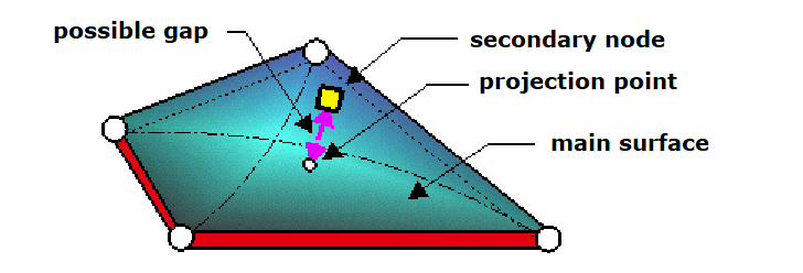
Figure 1.
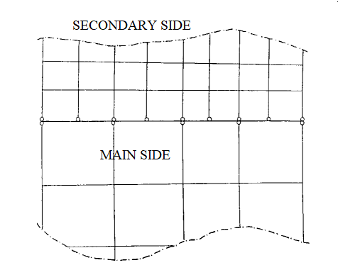
Figure 2. Fine and Coarse Mesh
A main and a secondary surface are defined in the interface input cards. The contact between the two surfaces is tied. No sliding or movement of the secondary nodes is allowed on the main surface. There are no voids present either.
It is recommended that the main surface has a coarser mesh.
Accelerations and velocities of the main nodes are computed with forces and masses added from the secondary nodes.
Kinematic constraint is applied on all secondary nodes. They remain at the same position on their main segments.
Tied interfaces are useful in rivet modeling, where they are used to connect springs to a shell or solid mesh.
Spotweld Formulation
- Default formulation
- Optimized formulation
Default Spotweld Formulation
- Based on element shape functions
- Generating hourglass with under integrated elements
- Providing a connection stiffness function of secondary node localization
- Recommended with full integrated shells (mainr)
- Recommended for connecting brick secondary nodes to brick main segments (mesh transition without rotational freedom)
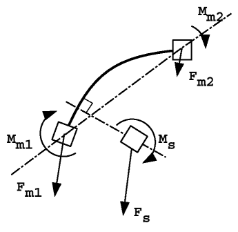
Figure 3. Default Tied Interface (TYPE2)
- Denotes the position of the secondary point
- Weight function obtained by the interpolation equations
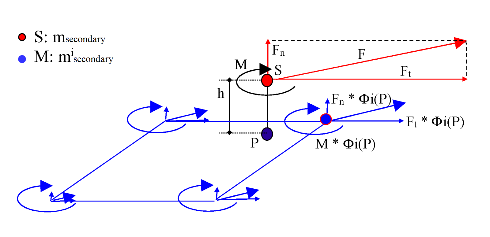
Figure 4. Transfer of Secondary Node Efforts to the Main Nodes (Spotflag=0)
The term may increase the total inertia of the model especially when the secondary node is far from the main surface.
With this formulation, the added inertia may be very large especially when the secondary node is far from the mean plan of the main element.
Optimized Spotweld Formulation
- Based on element mean rigid motion (i.e. without exciting deformation modes)
- Having no hourglass problem
- Having constant connection stiffness
- Recommended with under integrated shells (main)
- Recommended for connecting beam, spring and shell secondary nodes to brick main segments
This spotweld formulation is optimized for spotwelds or rivets.
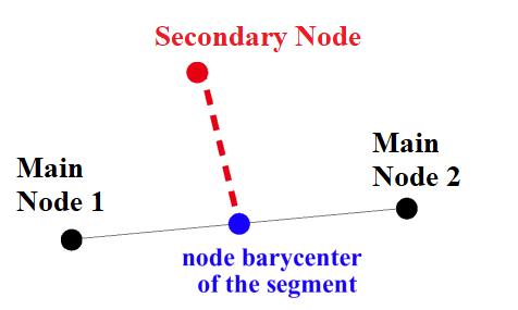
Figure 5. Relation Between Secondary Node and Main Node
- Normal vector to the segment
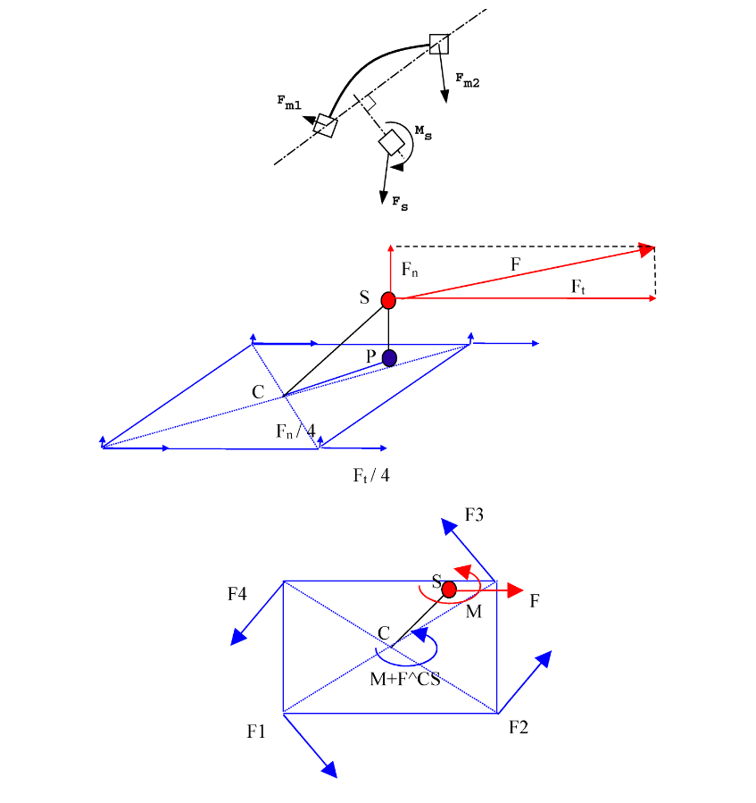
Figure 6. Optimized Tied Interface (TYPE2)
Closest Main Segment Formulation
- Old formulation
- New improved formulation
Old Search of Closest Main Segment Formulation
When Isearch= 1, the search of closest main segment was based on the old formulation.
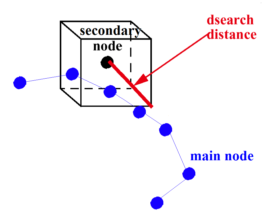
Figure 7. Old Search of Closest Main Segment
The distance between each main node in the box and the secondary node is computed.
The main node giving the minimum distance (dmin) is retained.
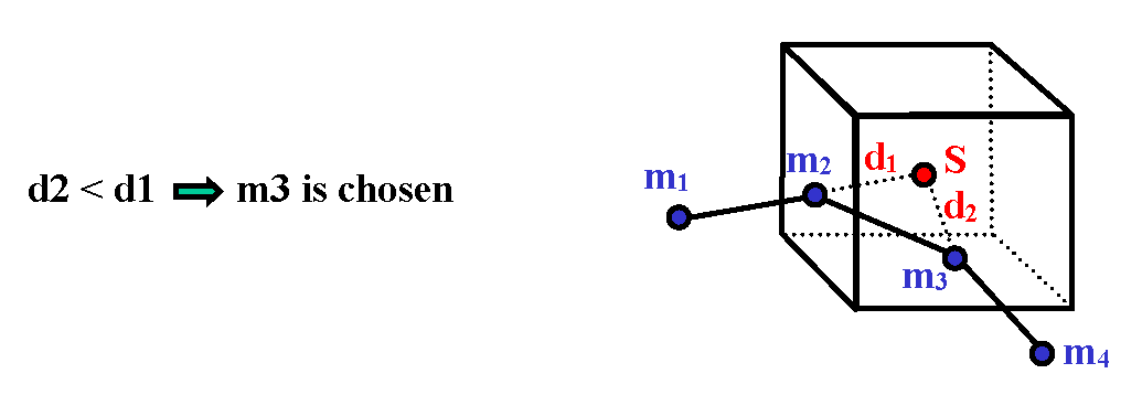
Figure 8. Old Search of Closest Main Segment
New Improved Search of Closest Main Segment Formulation
When Isearch=2, the search of closest main segment is based on the new improved formulation; a box including the main surface is built.
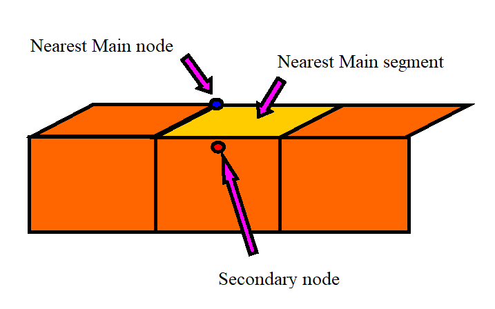
Figure 9. New Improved Search of Closest Main Segment
- The secondary node is an internal node for the main segment, as shown in Figure 10.The secondary node is projected orthogonally on the main segment to give a distance that may be compared with other distances. Select the minimum distance:
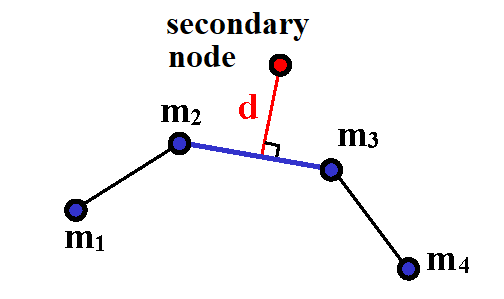 Figure 10. Orthogonal Projection on the Main Segment
The segment that provides the minimum distance is chosen for the following computation.
- The secondary node is a node external to the main segment, as shown in Figure 11.The distance selected is that between the secondary node and the nearest main node.
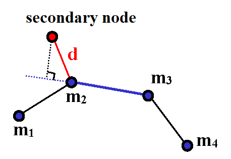
Figure 11. Nearest Main Node
The segment is chosen using the selected node, (if the selected node belongs to 2 segments, one is chosen at random).