Mesh Sensitivity

This typically entails solving for the pressure, velocity and turbulence fields within a given domain. These fields can be both spatially and temporally varying. To obtain a solution to the governing equations, the simulation domain is discretized into small, finite regions, referred to as elements or cells, that are made up of faces that are connected by nodes or vertices. The solver then solves the governing equations over each of these finite regions to approximate the solution over the whole domain. In the case of a finite element solver, the solution is obtained and stored at the nodal locations. In other words, the solution is permitted to vary at the locations of the nodes in finite element solvers. The solution between the nodal locations is assumed to vary linearly, in most cases. With this in mind, it is clear that the mesh resolution thus must be sufficient so that all variations in the flow are sufficiently captured by an assumed linear profile between the locations where the solution is stored. Mesh resolution is a measure of the distance between two consecutive measurement points in the mesh.

A consistent numerical analysis will provide a result which approaches the actual result as the mesh resolution approaches zero. In this case the elements become infinitesimally small and the mesh behaves almost like a continuous representation of the domain. Thus, the discretized equations will approach the solution of the actual equations. One significant issue in numerical computations is what level of mesh resolution is appropriate. This is a function of the flow conditions, type of analysis, geometry and other variables. An insufficiently resolved mesh that has nodes far apart will not capture the gradients well enough when assuming linear variations between nodes and will lead to a less accurate numerical solution. An unnecessarily finely resolved mesh will lead to higher solution costs without any gain in accuracy. You are often left to start with a coarse mesh resolution and then conduct a series of mesh refinements to assess the effect of mesh resolution. This is known as a mesh refinement study. Strategic mesh refinement will call for you running a solution on the coarse mesh, studying the results and identifying the areas that require enhanced resolution to improve the solution. The refinement process should be continued until the results do not change with further refinement. Such a solution may be referred to as the grid converged solution.

CFD practitioners must recognize the distinction between a numerical result which approaches an asymptotic numerical value and one which approaches the true solution. It is hoped that as the mesh is refined and resolution improves the computed solution will not change much and approach an asymptotic grid converged value, that is, the true numerical solution. However, there still may be error between this asymptotic value and the true physical solution to the equations. This behavior is shown in the image below.

Figure 1. Effect of Increasing Mesh Density on Accuracy of the CFD Solution

Each CFD solver has its own guidelines for what types of elements behave best from a stability, accuracy and convergence stand point. In addition to this, there are generally guidelines about the quality of each type of element that is suitable for use within the solver. Many finite volume solvers cite the aspect ratio of the elements, element skewness, orthogonality of the element faces and the element growth factor as critical metrics for determining their suitability for use. For this reason, it is sometimes recommended by code vendors that you use hexahedra elements for finite volume codes. Finite element solvers typically do not have this same constraint and will often recommend the use of tetrahedral elements. You should consider the needs of your solver when constructing a mesh to determine the most suitable discretization for your application.

The Backward Facing Step Case

The following example uses the backward step facing case. Consider a simulation of this flow using a CFD solver. Assume that you are creating a very coarse mesh on the geometry and then you are running a simulation. The CFD solver produces a solution to the Reynolds-averaged Navier-Stokes (RANS) equations on this discretization that results in a seemingly realistic flow field. The flow is characterized by the large separation zone downstream of the step and the recovering boundary layer after reattachment. Representative results for such a simulation are shown in the image below.

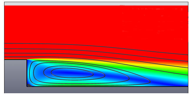
Figure 2. Streamlines Showing Separation Zone in Backward Facing Step Model

However, if there are insufficient points in the mesh to provide a good estimate of the gradients between the solution points the solver will not be able to resolve the flow features properly. Using this example, the shear layer that develops in the separation zone is under resolved and this leads to a poor representation of the reattachment point. In order to improve the solution it is necessary to refine the mesh in the locations of high velocity gradients. By doing this, the solver is better able to represent the local variations in the solution leading to a better approximation of the true solution to the governing equations. The image below shows five different meshes created for the backward facing step problem. Each mesh is progressively refined with respect to the previous mesh to illustrate the areas of refinement that must be paid careful attention to for this particular application.

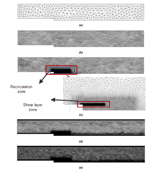
(a) Mesh 1; (b) Mesh 2; (c) Mesh 3; (d) Mesh 4; (e) Mesh5

Figure 3. Five Meshes Used in Backward Facing Step Mesh Sensitivity Study

The figure below shows the velocity profiles obtained from the solutions of each of the meshes using a consistent solver setup. Images (a) to (d) each correspond to the solution from mesh one through four, respectively. It is easy to see how the solution improves with each refinement in the mesh. A detailed discussion of these figures is covered in the mesh refinement process below.

Figures a-d each correspond to mesh one through four, respectively.

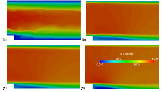
(a) Mesh 1; (b) Mesh 2; (c) Mesh 3; (d) Mesh 4

Figure 4. Velocity Profiles Downstream of the Step Depicting Mesh Sensitivity for the Backward Facing Step Case

It is evident that refining the mesh in the shear layer, recirculation zone and the near wall area where the velocity gradients are highest leads to a change in the solution between meshes one through four. However, it is interesting to note that as the mesh is further refined between grids four and five there is no change seen in the solution. This implies that the solution error associated with grid refinement has been minimized and you have reached an asymptotically grid converged solution with the mesh density and topology utilized in mesh four. All of the critical regions have been refined at this stage and suitable mesh topology as well as sufficient mesh resolution has been achieved. Further refinement of the mesh did not change the solution quantity of interest. A review of the table above indicates that the separation location changed by almost 50 percent between mesh one and the final grid converged solution of mesh four. If no grid sensitivity study was performed the engineer could have made very poor conclusions about the location of the pressure tap.

Appropriate grid refinement is one of the most important aspects of obtaining accurate CFD results. Unfortunately, there is currently no reliable method of automatically generating appropriate meshes for all applications. Additionally, different numerical methods will require different levels of mesh refinement, that is, each code will be different. Ensuring the suitability of a mesh for a given application is your responsibility. The level of accuracy required from a CFD analysis depends on the desired use of the results. A conceptual design effort may be content with general depiction of the flow features, whereas a detailed design may require accurate determination of the flow field. Each quantity to be determined generally has its own accuracy requirement. Levels of effort invested into the CFD model may vary according to the information required. It is often recommended that a minimum of three different meshes are constructed that cover a wide range of refinement and differ significantly in mesh density and resolution. For applications that require high levels of accuracy this number may be more depending on the number of mesh refinements it takes to achieve a grid converged solution. This allows you to evaluate the sensitivity of the solution quantity of interest to mesh density. Some CFD practitioners endorse the use of a Grid Convergence Index, or GCI, to estimate the level to which a simulation has reached a grid independent solution. More information about the GCI metric is available in the book by Patrick J. Roache, listed in reference [1].