Convergence Sensitivity
This section discusses and illustrates the effects of the level of convergence tolerance you provide to the solver, and also stresses on the need to look for other solution parameters before accepting a solution.
The convergence of the CFD solver gives an indication of how well it has solved the discretized equation set for the application of interest. Most CFD solvers measure convergence by monitoring the residuals, which represent the imbalance of terms in the governing equations at each iteration. As a general rule, the lower the residuals the lower the error due to imbalance in the terms in the equation. Some solvers also monitor the degree to which the solution is changing between iterations. As the simulation progresses, the residuals should fall and also the solutions to the equations should reach a stabilized value. It is a good practice to measure a solution quantity which may also capture the behavior of other solution variables to determine convergence. A converged solution means that the solver has done its job and produced the best solution it can for the given setup. However, that does not guarantee that the solution is correct in comparison to test or physics. The accuracy of the solution is a function of many other characteristics, some of which are described above.
CFD solver packages typically set default convergence criteria that are suitable for many applications. However, if high levels of accuracy are important it is necessary to monitor the impact of convergence on the solution for the application of interest. For steady state simulations this means monitoring the solution quantity of interest as the simulation is converged further. For transient applications it is also necessary to evaluate the convergence at each time step to see how it impacts the overall transient.
The Backward Facing Step Case
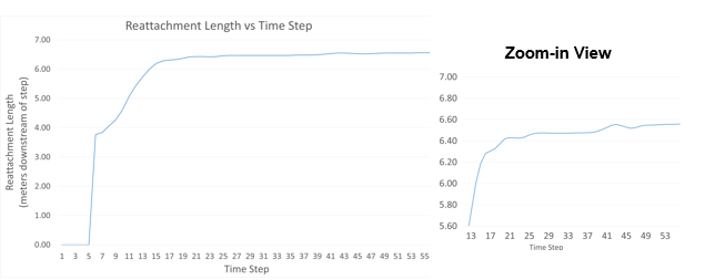
Figure 1. Convergence of Backward Facing Step Model
A closer inspection of the reattachment length convergence history in the second plot shows that the size of the separation zone does not stabilize until about time step 42. Therefore, the level of convergence necessary to obtain a high level of accuracy for the separation location corresponds to the levels corresponding to step 42 of the simulation. This value may or may not coincide with the solver's default convergence tolerance settings.
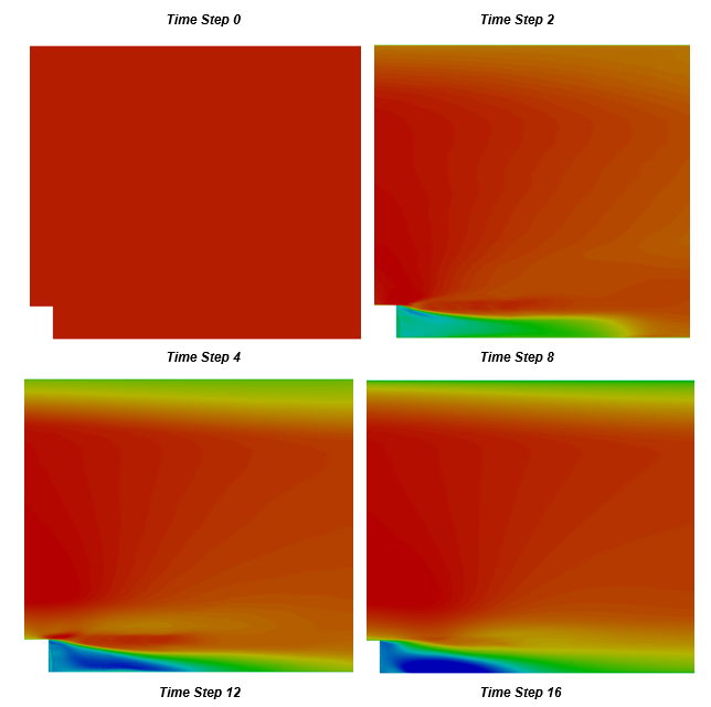
Figure 2. Convergence Behavior of the Backward Facing Step Simulation using the Shear Stress Transport (SST) Turbulence Model
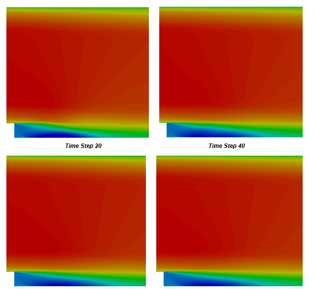
Figure 3. Convergence Behavior of the Backward Facing Step Simulation using the SST Turbulence Model
Each solver will be different and will perform differently on each application. It is up to you to investigate the proper convergence levels for your application. It should also be noted that convergence cannot be gauged by the residual metrics alone. Judging suitable convergence levels involves monitoring the convergence metrics, the solution quantity of interest, as well as looking at momentum and mass balances within the flow field when possible.