ERROR_ESTIMATOR_OUTPUT
Specifies parameters for outputting the nodal error estimator.
Type
AcuSolve Command
Syntax
ERROR_ESTIMATOR_OUTPUT {parameters}
Qualifier
This command has no qualifier.
Parameters
- type (enumerated) [=pde_residual]
- Which error estimator to use.
- pde_residual or pde_res
- Error estimate base on equation residual.
- output_frequency or out_freq (integer) >=0 [=0]
- Time step frequency at which to output the error estimator. If zero, this option is ignored.
- output_time_interval or out_intv (real) >=0 [=0]
- Time frequency at which to output the error estimator. If zero, this option is ignored.
- num_saved_states or save (integer) >=0 [=0]
- Number of error estimator files to keep. If zero, all error estimator files are kept.
- time_average_output_frequency or ave_out_freq (integer) >=0 [=0]
- Time step frequency at which to output the time average of the error estimator. If zero, this option is ignored.
- time_average_output_time_interval or ave_out_intv (real) >=0 [=0]
- Time frequency at which to output the time average of the error estimator. If zero, this option is ignored.
- num_time_average_saved_states or ave_save (integer) >=0 [=0]
- Number of time average of the error estimator files to keep. If zero, all time average of the error estimator files are kept.
- time_average_reset_frequency or ave_reset_freq (integer) >=0 [=0]
- Time step frequency at which to reset the averaging process. If zero, never reset.
Description
 , of
GLS stabilization terms. Hence, these residuals are not expected to go to zero with
solver convergence. For
example,
, of
GLS stabilization terms. Hence, these residuals are not expected to go to zero with
solver convergence. For
example,ERROR_ESTIMATOR_OUTPUT {
type = pde_residual
output_frequency = 100
output_time_interval = 0
num_saved_states = 2
}writes a nodal error estimator file to disk every 100 time steps as well as the last time step. Only the last two files are kept. Once the third nodal error estimator file is written to disk, the first nodal error estimator file is removed to preserve disk space.
ERROR_ESTIMATOR_OUTPUT is an advanced command that can be used to evaluate the quality of the mesh or problem modeling.
If either output_frequency or output_time_interval is non-zero, an error estimator file will be written at the end of the run. If both are zero, no error estimator files are created.
Run times may not coincide with output_time_interval. In this case, at every time step which passes through a multiple of output_time_interval, an error estimator file is written.
The num_saved_states parameter indicates the number of nodal error estimator files to save. Once the (num_saved_states + 1)th nodal error estimator file is written, the first one is removed. When running in parallel, once all files are written (in parallel), then the old ones are removed (in parallel).
ERROR_ESTIMATOR_OUTPUT {
   type                              = pde_residual
   time_average_output_frequency     = 100
   time_average_output_time_interval = 0
   num_time_average_saved_states     = 2
   time_average_reset_frequency      = 10
}
Here, the error estimator is averaged over 10 steps before it is output.
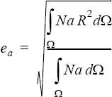
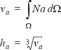
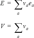
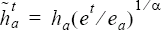
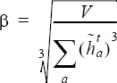
where ea is the error estimator at node
a, R is
the residual of one of the differential equations (mass, one of the momentum
equations, heat, one of the species equations, or turbulence) and the corresponding
least-squares metric,  , of
GLS stabilization terms, Na is the
shape function for node a, and Ω is volume.
, of
GLS stabilization terms, Na is the
shape function for node a, and Ω is volume.