HG-1011: Perform Math on Curves Using the Plot Browser
In this tutorial, you will learn how to use the Plot Browser to perform math on a single curve in the Define Curves panel without creating duplicate curves and to apply this math to all other curves in the session via the Plot Browser.
The HyperGraph 2D Plot Browser resides on a tab in the Tab Area sidebar and allows you to view the HyperGraph 2D plot structure.
The Plot Browser can be turned on or off using the menu options. A check mark indicates that the HyperGraph 2D Plot Browser is activated for display in the Tab Area.
You can use the Plot Browser tools to search, display and edit entities and their properties within the current session.
From the Define Curves panel, you can edit existing curves and create new ones. To edit a curve, it must first be selected either from the curve list or picked from the window.
The X,Y, U, and V vectors are displayed at the top of the Define Curves panel. The data sources for these vectors are displayed in the text fields. Click the radio button for a vector or click in the corresponding text box to select that vector for editing. In addition to the traditional X and Y vectors, you can perform math on curves prior to plotting your data with the support of u and v vectors. As a result, only one curve is generated in the session, whereas in the older versions of HyperGraph, this could not be done without an initial curve.
To use math as a data source, from the Define Curves panel, select .
Open Session File demo_browser.mvw
- From the File menu, click .
- From the plotting folder, select the demo_browser.mvw file and click Open.
Use the Define Curves Panel to Apply an SAE Filter to a Curve
-
From the toolbar, select the Define Curves icon,
 .
.
You can now apply math to the y vector.
-
From the Functions dialog, select
saefilt95 and click OK.
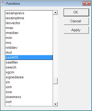 Figure 1.
 -
The result is a corrupt curve. This is because the function expects the time to
be in seconds, and our curve is in milliseconds.
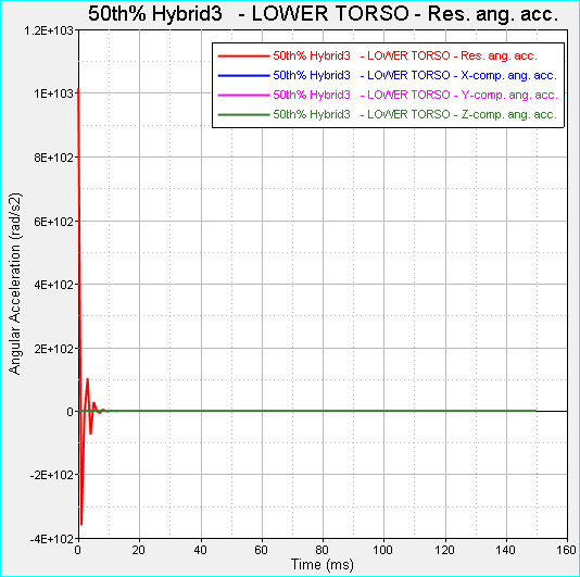 Figure 2.
 -
To correct this, you must apply the time vector by 0.001. Enter the following
in the y= field: saefilt95(u*0.001,v,60,20,3).
The result is a properly filtered curve:
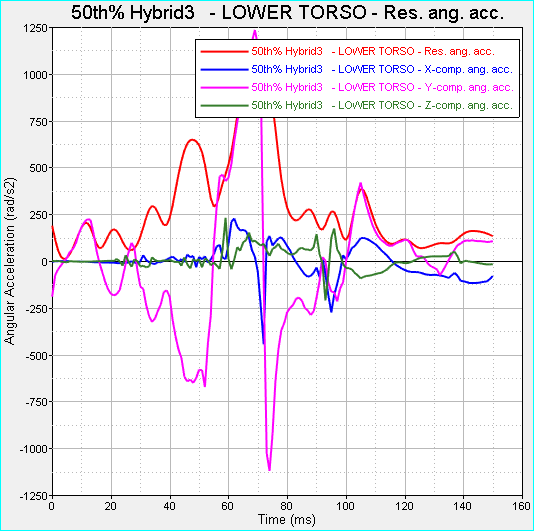 Figure 3.
Apply the Math Performed in Step 2 to all Other Curves in the Session Via the Plot Browser
In this step, you will apply the filter defined in Step 2 to all curves in the session using the Plot Browser.
-
As shown below, right-click on the y vector and select Select
All.
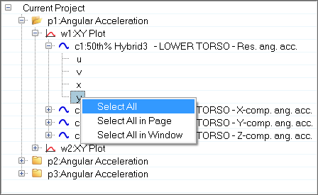 Figure 4.
 All y vectors in the session are selected.
-
Notice that all the curves in the graphics area disappear, except for the curve
we have already filtered on the Define Curves panel.
 Figure 5.
 -
Click in the Expression field and paste the filter you copied from the Define
Curves panel and press Ctrl.
All curves in the session now contain the same filter and math.
 Figure 6.
 -
In the Expression field, enter u.
Now all vectors in the session have the same math.
 Figure 7.