Data Sources
Curves are comprised of an X data vector and a Y data vector. The X and Y vectors can be read from a data file, defined as mathematical expressions, or entered as values. The X and Y vectors of a curve do not have to come from the same source. For instance, the data source for the X vector of a curve can be an ASCII file and the source for the Y vector of the same curve can be defined by an expression such as sqrt(x).
File as a Data Source
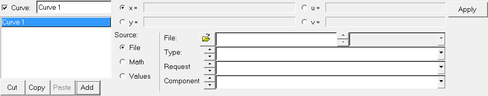
Figure 1.
Math as a Data Source
If Math is selected as the source, the curve calculator is displayed, allowing you to define the vector mathematically.
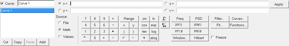
Figure 2.
- Curve Calculator
- Curves can be defined mathematically using the curve calculator.
- Range
- Defining a range is a quick way of specifying a spread of values for a vector. Click Range to display the Range dialog.
- Calculus Functions
- Integrals and derivatives are displayed
as:
integral(,)
derivative(,)
Independent and dependent vectors must be supplied for both functions.
See Math Reference for a detailed description of each function and its purpose.
- Signal Processing
- Fast and discrete Fourier transforms, as well as windowing, power spectral density, and frequency response functions can be included in expressions.
-
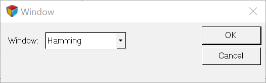
Figure 3. - Filter
- Curves may be passed through two classes of filters, ideal or SAE. Click Filters... to display the Filter dialog box.
-
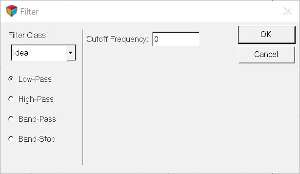
Figure 4.Select either Ideal, SAE or SAE J211/1 from the Filter Class option menu.
There are four ideal filter types available:- low pass
- high pass
- band pass
- band stop
For ideal filters, specify the type of filter and the cutoff frequency. Band pass and band stop filters require both a low and a high cutoff frequency. Click OK to insert the filter into the expression.
Any SAE filter class can be specified by modifying the entered filter class (60, 180, 600, or 1000) in the Y text field.
For SAE J211/1, select the padding type and direction.
- Fit
- Polynomial and exponential functions can be fit to curves. Click Fit... to display the Curve Fit dialog box.
-
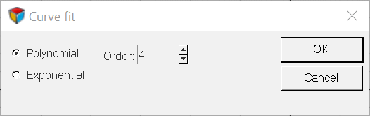
Figure 5. - Math Functions
- The Functions... button displays a dialog box containing all available
math functions. External functions or Templex functions can be registered in the program using
*RegisterExternalFunction() or
*RegisterTemplexFunction() in the preference
file.
Any of the functions can be inserted into the current expression by selecting the function name from the list or by typing the name directly into the equation.
See the List of Standard Functions topic in the Math Reference help for more information.
- External Functions
- In addition to the built-in math functions and operators, external C-programs can also be called from within a math expression.
- Freezing Vectors
- When a vector is defined by an expression, the program automatically
recalculates the vector each time the expression is altered, in turn,
updating the curve. If an expression contains a reference to another
curve and the referenced curve changes, the program recalculates the
vector and updates the curve containing the reference.
Vectors can be frozen so that the program does not recalculate the curve. When a vector is frozen, it is no longer dependent on a referenced curve, so changes made to other curves are not reflected in the frozen vector. Vectors can be unfrozen, making them once again subject to change. The X and Y vectors can be frozen independently of each other or together, freezing the entire curve. Frozen vectors are saved as data point values in session files.
Values as a Data Source
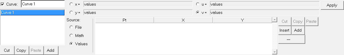
Figure 6.