Non Systematic Issue / Free Size Optimization
The advantages of choosing free size optimisation are as follows:
- Free-size optimization (targeting Non-Systematic issues) in OptiStruct optimizes the thickness of every element in the design space to generate an optimized thickness distribution in the structure, for the given objective under given constraints.
- In SnRD Modal Frequency Response analysis is used as the optimization load case with an objective of minimizing the modal relative displacement across the selected E-Line.
- SnRD Optimization module automatically converts the time domain excitations to frequency domain for creating the MFREQ loadcase. Amplitude and phase are considered.
- The design variable for free-size optimization is the thickness of the shell elements on the surfaces.
- Optimization can be done for the response at single frequency or for a band of frequencies.
The work flow of the Free-size optimization (Non-Systematic Issue) is illustrated below:
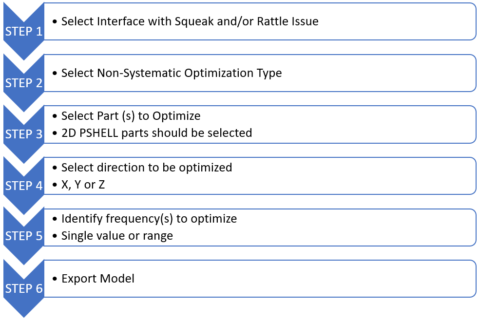
Figure 1.
Optimisation Deck setup
Once the optimization deck setup is initiated, following changes are done to the solver deck:
- Load case setup : Modal Transient (MTRAN) analysis is changed to Modal Frequency Response (MFREQ)
- Optimization parameters set-up: Responses and Constraints
Optimization Deck Setup process
Steps for setting up Optimization deck are given below:
- Select the required loadcase.
- Select interface with Squeak and/or Rattle issue.
- Load the interface to understand the critical frequencies.
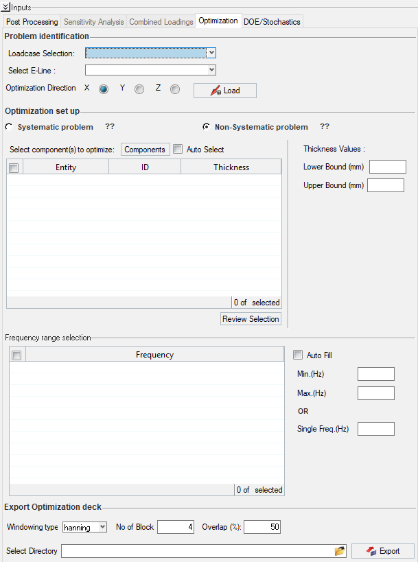
Figure 2.Note: HyperView window splits into four:- .h3d file of Modal Transient analysis, showing selected interface and all 2D parts.
- Relative displacement graph for selected interface.
- Relative Modal Contribution bar chart.
- .h3d file of modal analysis
- Select Optimization type as Non-Systematic Problem.Note: By default the option is Systematic Problem.
- Select Part or Parts to Optimize. Select the Auto Select check box to automatically select the components related to the selected interface.
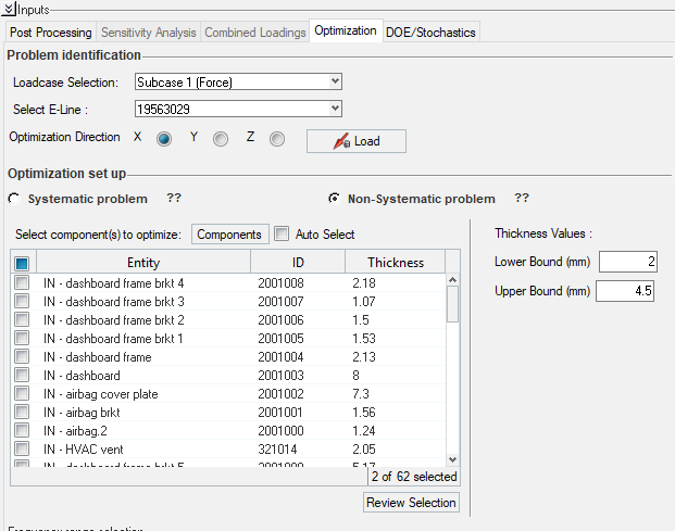
Figure 3.The 2D PSHELL parts must be selected.Note:- Only 2D PSHELL parts must be selected.
- A part list is populated with the parts to be optimized.
- Automatic selection of 2 Parts based on the interface selected using the associated part selection.
- Ability to adjust (add/remove) selected part list.
- Identify frequency or frequencies to optimize.
- Select the Auto Fill option to automatically fill the frequency (Top Contributing mode
from RMC Bar Chart) or frequencies of selected modes.
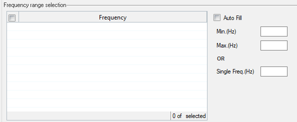
Figure 4.Note: Frequency range selection table will be empty for a Static Load case setup work flow.
Steps to export solver deck are given below:
- Fast Fourier Transformers definition options are available in the Export
Optimization deck
- Windowing Type - As you may be aware, a typical modal
transient run is time based analysis. For optimizing the E-line for systematic or a
non-systematic optimization problem in the frequency domain , we need to convert the
time domain data in the input deck to the frequency domain. Altair Compose takes care
of this conversion in the back end using some of the basic inputs required for the FFT
(Fast Fourier transform). These inputs are now available in the interface to modify.
Based on the type of windowing option in time to frequency conversion, the default
parameters automatically populate.
- Uniform -
- Hanning -
- Number of Blocks - We perform a block based FFT where the signal is processed by breaking it into given no of blocks and suitable windowing technique is used to reduce the effects of the leakage.
- Overlap(%) - Overlap percentage is also a measure to reduce the truncation effects. The overlapping windows with suitable windowing type like hanning or uniform helps in providing smooth transition from one block to the next. Refer to textbooks for more details on these inputs.
- Windowing Type - As you may be aware, a typical modal
transient run is time based analysis. For optimizing the E-line for systematic or a
non-systematic optimization problem in the frequency domain , we need to convert the
time domain data in the input deck to the frequency domain. Altair Compose takes care
of this conversion in the back end using some of the basic inputs required for the FFT
(Fast Fourier transform). These inputs are now available in the interface to modify.
Based on the type of windowing option in time to frequency conversion, the default
parameters automatically populate.
- Click file browser icon for Select Directory option.

Figure 5. - Click Export button.