The MoM is the default solver in Feko. A simple electrostatic example is used to convey the basics of the
solver.
The Charge Distribution of a Straight Wire at a Constant Electric Potential of 1
V.
The basic Yagi-Uda antenna shown in Figure 5 consists of a few
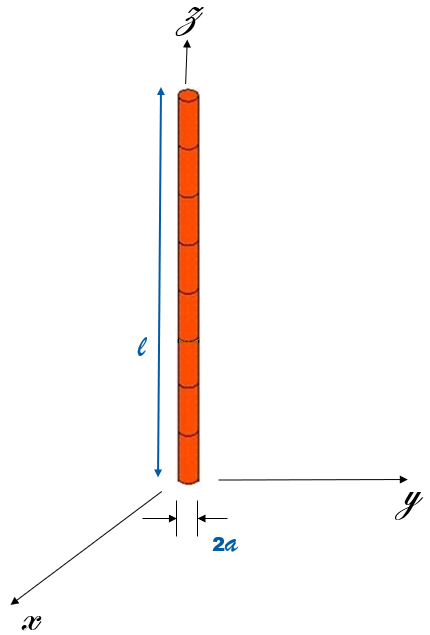
straight wires. Consider the solution of the charge distribution of a single straight wire
of length and diameter 2a shown in Figure 1.
Figure 1. A segmented straight wire charged to a constant potential.
According to 1, a linear electric charge distribution will create an electric potential as follows:
(1)
where represents the source coordinates and r denotes the
observation coordinates, is the path of integration and R is the distance from
any point on the source to the observation point which can also be written as
(2)
Note:Equation 1 is valid on the
wire and in free space. This is the so-called "boundary condition" for this particular
problem.
Even though the charge distribution on arbitrarily shaped objects are not generally known,
the straight wire example is useful for an introduction to the MoM.
Assume the wire is charged to a constant electric potential of 1 V. For convenience, the
wire is oriented parallel to the Z axis. To solve Equation 1 on a computer, the
wire is divided into smaller segments and the charge distribution can be approximated as
follows:
(3)
The functions, , often referred to as basis functions, are chosen to
accurately model the unknown quantity (here the charge on a wire segment) as well as for
computational efficiency. For simplicity, constant functions over each segment are assumed.
More specifically, each function is equal to 1 over one segment only, and zero
elsewhere. The assumption of a constant function implies that the segment length should be
short enough for this assumption to hold.
Note: A rule of thumb is to make segments th of a wavelength.
Therefore Equation 1 can be
approximated as follows:
(4)
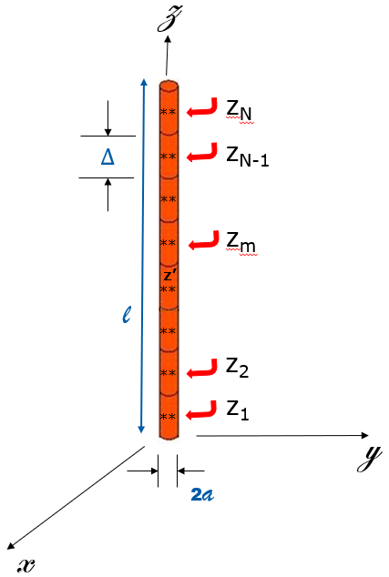
As shown in Figure 5, the
wire is divided into N uniform segments where each segment is of length .
Figure 2. A segmented straight wire charged to a constant potential.
Since Equation 1 is valid
everywhere, z can be chosen to be located at fixed points, zm, on
the surface of the wire segments with radii, a. This choice simplifies Equation 4 to only a function
of z', allowing the calculation of the integral. Furthermore, since the wire was
divided into N segments, Equation 4 can be written as one equation with N unknowns
(an) as follows:
(5)
An equation of N unknowns requires N equations where each equation stands
linearly independent from each other. These N equations can be constructed by
selecting the observation points zm in the centre of each segment of
length as shown in Figure 2.
Note: The selection of observation points is denoted
“testing” or “sampling” and the method is referred to as “point-matching” or
“collocation”.
Performing the selection of points N times reduces
Equation 5 to the
following:
(6)
Equation 6 can be more
readily written in matrix form as:
In addition, we can write the remaining two terms:
(9)
(10)
The Vm matrix consists of 1 row and N columns and all entries are
equal to . The an values are the unknown coefficients
for the charge distribution. To solve Equation 7, the matrix
requires inversion where
(11)
Note: A well-known and computationally cheaper inversion
procedure, LU decomposition, is followed. The matrix is factored into an upper and lower
triangular matrix. Then a process similar to Gaussian elimination is followed to solve the
matrices.
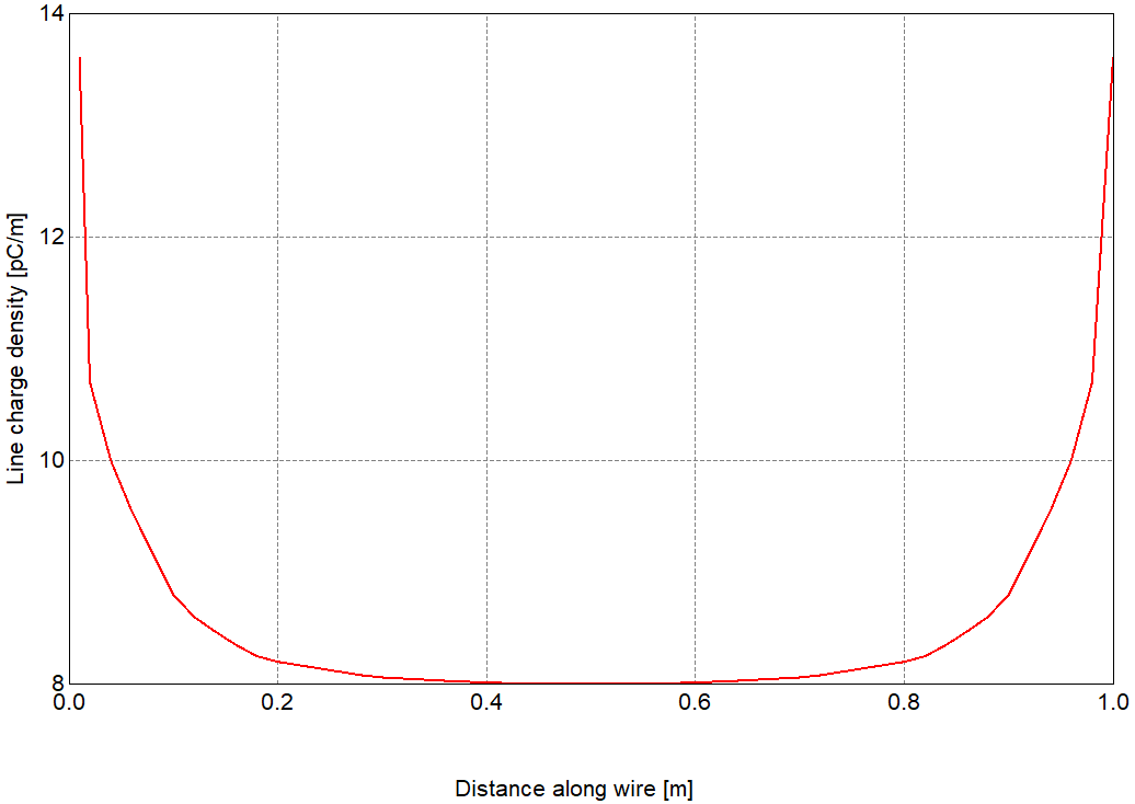
Figure 3 shows the line charge
density for a wire of length 1 m discretized into 50 segments.
Figure 3. Line charge density of a straight wire charged to a potential of 1 V.
For more complex problems, the integrals cannot be reduced to approximations such as those
made here.
1 Advanced Engineering Electromagnetics, Second Edition, Constantine A.
Balanis, p. 680