Basic Concepts
Basic antenna and EM concepts are given that provide a foundation for understanding the different solver methods in Feko.
What is an Antenna?
An antenna is a conducting structure consisting of surfaces and/or wires designed to be of specific characteristic dimensions to radiate or receive an electromagnetic wave.
The primary purpose of an antenna is to make an impedance match between a signal (electrical current or wave) travelling in a coaxial cable (transmission line) or wave guide and waves travelling in free space. A secondary purpose is to send the signal in a specific direction. 12
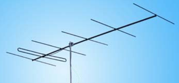
Figure 1. A Yagi-Uda antenna.
What is a Far Field?
- Differences in the distances from P to the different points on the radiator have a negligible effect on the magnitude of the field.
- Differences in the distances from P to the different points on the radiator should be accounted for when calculating the phase, but certain assumptions could be made.
- All field components that decay faster than can be considered negligible compared to those that decay with .3
The far field of an antenna is the minimum distance from the antenna where the field components do not contain reactive components, or where these components can be considered negligibly small. This distance is generally written as:
where D is the largest dimension of the antenna.
In the far field, the antenna is considered a point source. Equation 1 is derived under the assumption that the varying distances to the radiator do not contribute to phase errors larger than 22.5°.4
What is a Near Field?
The near field of an antenna is the region in close proximity to the antenna where the electric and magnetic fields are not in phase. The fields are reactive and there is also a strong radial component. The radial component of the field has no dependency but does have , and even higher dependencies. Naturally, these field components vanish very quickly with increasing distance.5
What is a Transmission Line?
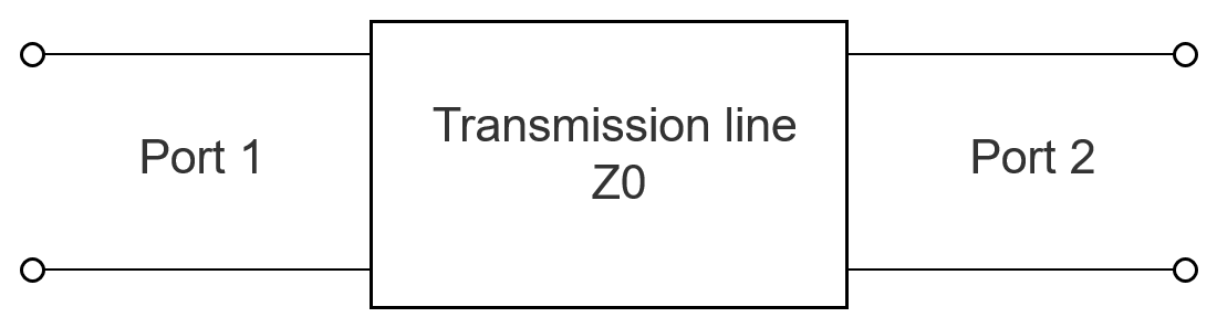
Figure 2. A basic representation of a transmission line.
From a radio frequency engineering point of view, typical parameters of interest are the input reflection coefficient and the voltage standing wave ratio (VSWR).
What are S-Parameters?
S-parameters characterize the relationship between the input and output ports of a system in terms of power waves. While the relationship could also be described in terms of other network parameters such as ABCD, Z and Y-parameters, calculating these parameters require the termination of the ports in open or short circuits. Achieving purely open or short circuits, especially over wide bands, are not feasible. In addition, some devices are not stable if they are open or short-circuited.
However, when calculating S-parameters, it only requires termination of the ports in the system impedance.6
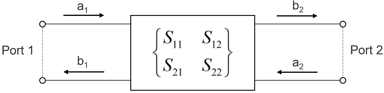
Figure 3. Two-port S-parameters representation.
What is the Reflection Coefficient?
The reflection coefficient is a quantity or figure describing how much of an electromagnetic wave is reflected due to an impedance mismatch (discontinuity) in the transmission line or transmission medium. The reflection coefficient is calculated as the ratio of the magnitude of the reflected wave to the incident wave. It can be calculated from the characteristic impedance of the transmission medium (line), , and the impedance of the discontinuity (often the load impedance at the end of a transmission line), , as follows:
What is a Smith Chart?
Figure 4. An empty Smith chart from POSTFEKO.
What is CEM?
Computational electromagnetics (CEM) refers to a numerical solution or a computer-based approximation of the currents or the fields. In the numerical solution the currents or fields are firstly divided into many small parts. Subsequently the physical equations (typically Maxwell's equations such as Ampère's law, Faraday's law) that describe the relationships between fields, currents and charges are then used to obtain the magnitude and phase of each current or field element. Finally the summing (integration) of these current or field elements yield antenna parameters such as input impedance and far fields.
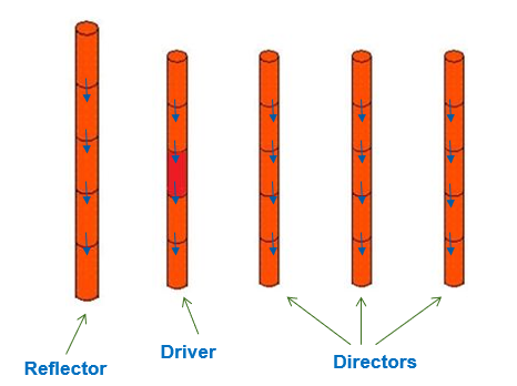
Figure 5. A Yagi-Uda antenna, current-carrying parts only, divided into small sections with uniform current elements across the junctions.
It is initially assumed that on each junction between sections, a constant current is flowing, but the magnitude and phase of these currents are not known. Maxwell's equations are used to find the magnitude and phase of each small current element.
Once the magnitude and phase of each current element is known, all the currents are added together (integrated). A transformation of the currents then give the electric and magnetic near and far fields as well as other antenna parameters.
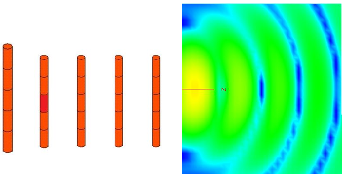
Figure 6. Yagi-Uda antenna near fields visualised in POSTFEKO.