Feko is a comprehensive electromagnetic solver with multiple solution methods that is used for electromagnetic field analyses
involving 3D objects of arbitrary shapes.
3D views are used to display and interact with the model. You can zoom, rotate and pan around a 3D model using the keyboard,
mouse or a combination of both. You can use a 3D mouse, specify a view or select specific parts of a model. Multiple 3D
views are supported.
Define field or current data using either far field data, near field data, spherical mode data or PCB current data. The
field/current definition is used when defining an equivalent source or a receiving antenna.
Define a medium with specific material properties, import a predefined medium from the media library or add a medium from
your model to the media library.
Defined media can be applied to the model in various ways. Some media settings are applied to regions, others on faces
and wires. The rules for defining media varies between the different solution methods.
Use a periodic boundary condition (PBC) to analyse infinite periodic structures. A typical application of PBC is to
analyse frequency selective surface (FSS) structures.
Create an arbitrary finite antenna array that consists of an array of contributing elements, either with direct feeds for
each element or via indirect coupling, and solve with the efficient domain Green's function method (DGFM).
Use the windscreen tools to define a curved reference surface constrained by a cloud of points, normals and optional U′V′ parameters. The constrained surface is then used as a reference to create a work surface where windscreen layers and curved
parameterised windscreen antenna elements can be created.
Many electromagnetic compatibility and interference problems involve cables that either radiate, irradiate or cause coupling
into other cables, devices or antennas. Use the cable modelling tool and solver to analyse the coupling and radiation.
For a frequency domain result, the electromagnetic fields and currents are calculated at a single frequency or frequency
range. When the finite difference time domain (FDTD) solver is used, the frequency must be specified to convert the native time domain results to the frequency domain.
The excitation of an antenna is normally specified as a complex voltage, but it may be useful to specify the total radiated
or source power instead. The result is then scaled to yield the desired source power level.
A port is a mathematical representation of where energy can enter (source) or leave a model (sink). Use a port to
add sources and discrete loads to a model.
Obtain multiple solutions for a single model using multiple configurations. Multiple configurations remove the requirement
to create multiple models with different solution requests.
Use an infinite plane or half-space to model a ground plane efficiently. The number of triangles in the model is reduced
as the ground plane is not discretised into triangles.
A CADFEKO.cfm file can be imported into EDITFEKO to make use of more advanced features available in EDITFEKO and to directly edit the .pre file for more flexible solution configurations.
During the design process, the development of a model can introduce a range of issues that can lead to a non-simulation-ready
model. Use the validation toolset to verify that the model is simulation-ready or to search, detect and flag discrepancies.
Before running the Solver, run the CEM validate tool to perform basic consistency checks on the model. These checks are largely related to
basic electromagnetic modelling rules and limitations (but not mesh parameters).
When defining a windscreen, the layer thickness is not displayed by default. Enable the windscreen layer thickness
to visually verify that the model is correct.
A cutplane is a display option that creates a plane at a designated location that cuts through an object to create a sectional
view. Create multiple cutplanes to create a sectional view that exposes inner details that would otherwise not be visible
from outside the model.
Before running the Solver, you can verify that the correct solution settings are applied to the geometry. Use the tool to highlight all the relevant
geometry in the 3D view with a specific solution method applied.
After applying union or stitching operations, you can verify that all the intended edges are connected. A face with unbounded
edges is an indication of unconnected mesh.
The default solver used in Feko is the method of moments (MoM) - surface equivalence principle (SEP). Whether a solver is specified per model, per face or per region, depends on the solver in question.
CADFEKO has a collection of tools that allow you to quickly validate the model, for example, perform calculations using
a calculator, measure distances, measure angles and export images.
EDITFEKO is used to construct advanced models (both the geometry and solution requirements) using a high-level scripting language
which includes loops and conditional statements.
One of the key features in Feko is that it includes a broad set of unique and hybridised solution methods. Effective use of Feko features requires an understanding of the available methods.
Feko offers state-of-the-art optimisation engines based on generic algorithm (GA) and other methods, which can be used
to automatically optimise the design and determine the optimum solution.
Feko writes all the results to an ASCII output file .out as well as a binary output file .bof for usage by POSTFEKO. Use the .out file to obtain additional information about the solution.
CADFEKO and POSTFEKO have a powerful, fast, lightweight scripting language integrated into the application allowing you to create
models, get hold of simulation results and model configuration information as well as manipulation of data and automate
repetitive tasks.
During the design process, the development of a model can introduce a range of issues that can lead to a non-simulation-ready
model. Use the validation toolset to verify that the model is simulation-ready or to search, detect and flag discrepancies.
An item is marked suspect when changes in the model result in the settings of an item
becoming unresolved or invalid.
A suspect item is indicated by a icon in the
model tree or details tree. Move the mouse cursor over the icon to
view the tooltip and the reason why it is marked suspect.
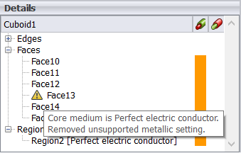
Figure 1. An example of a suspect item and its tooltip in the model tree.
Examples of situations where items can become suspect;
If a lossy conducting surface is set on a face bordered by free space and one of the
bordering regions is set to PEC, the unsupported metallic is removed. The face is marked
“suspect” and its medium displayed as PEC in the details tree.
If a port becomes invalid due to a change in the model, the port is marked
“suspect”.
Note: Resolve all suspect items before launching the Solver or OPTFEKO. The loss of properties on the model geometry may change the
electromagnetic problem description and impact the computed results.
Tip: Remove the suspect icon by ensuring that the properties on the item are
correct. From the right-click context menu select Set not
suspect.