Apply a varying pressure load to full or partial face(s) of revolution.
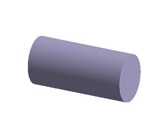
Examples of supported face types, such as cylindrical, conical, concave torus
and so one, are shown below.
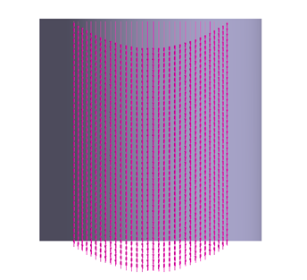
Cylindrical
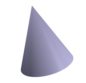
Conical
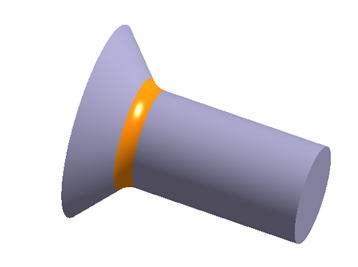
Concave torus
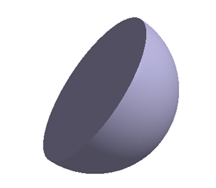
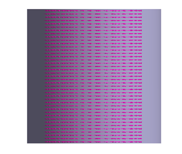
Other
You can apply loads on multiple faces of the same part. You can
apply bearing loads as forces in radial and axial directions, and as torque to the
selected faces.
Radial Force
Axial Force
Torque
For dynamic analyses, each load must
reference a time/frequency function curve.
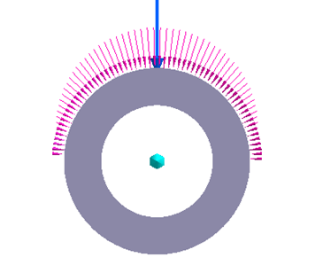
The faces may be concave (as shown in Figure 1) or convex (as shown in
Figure 2). Figure 1. Figure 2.
In the Project Tree, open
the Analysis Workbench.
In the workbench toolbar, click the (Bearing load) icon.
In the modeling window click to select a face of
revolution on the model.
The selected point on a face of revolution will indicate load
direction.
Tip:
The axis about which the bearing load is applied is calculated based on
the initial face picked in the graphics. After the axis of the load is
determined, you can pick a face of any type.
Under Load, specify the numerical value and the units for radial, axial, and
torque loads.
Use the Radial Direction and Span fields to adjust load
direction.
Note: You can also adjust the load direction using the Degree field or by
entering a reference XYZ vector direction.
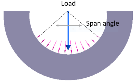
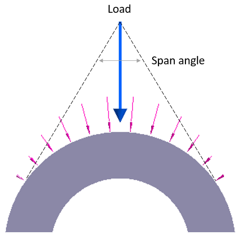
Specify the Load span angle.
Note: Valid load span angles are 10 to 180 degrees.
Click Apply.
The load is applied as a pressure, whose magnitude is spread using a
sinusoidal distribution over the Load span angle. In Non-linear
Structural analysis, bearing pressure is assumed to be a follower load
as it follows the Part geometry change when large deformations occur.
Pressure always remains normal to the deformed face of a Part.
 (Bearing load) icon.