In this tutorial, you will learn how to create an analysis definition and instantiate
it in an MDL file.
An analysis is a collection of loads, motions, output
requests, and entities (bodies, joints, and so on) describing a particular event applied
to a model. For example, an analysis to determine the kinematics of a four-bar mechanism
can be described in one analysis, while another analysis can be used to study a dynamic
behavior. In both cases, while the overall model is the same, the analysis container may
contain different entities that form the event. The kinematic analysis can contain
motion and related outputs, while the dynamic analysis may contain forces and its
corresponding outputs.
An analysis definition is similar to a system definition in
syntax and usage except for these key differences:
Analysis definitions use *DefineAnalysis(), while system
definitions use *DefineSystem().
Analysis can be instantiated under the top level Model only.
Only one analysis can be active in the model at a given instance.
An analysis definition block begins with
*DefineAnalysis() and ends with
*EndDefine(). All entities defined within this block are
considered to be part of the analysis definition. The syntax of
*DefineAnalysis() is shown
below:
ana_def_name The variable name of the analysis definition
which will be used while instantiating the analysis.
arg_1,arg_2...arg_n A list of arguments passed to the
analysis definition as attachments.
Table 1
illustrates an analysis definition and its subsequent instantiation within an MDL
file. Two files, an analysis definition file and the model file, work together when
instantiating a particular analysis under study. Some of the terms in the example
are in bold to highlight a few key relationships between the files.
Table 1.
Reference Numbers
System Instantiation with Definition
1
// Model : Body.mdl
*BeginMDL(base_model, "Base Model")
2
//Instantiate the analysis definition ana_def
*Analysis(ana1, "Analysis 1", ana_def, j_rev)
//Declare a joint attachment to the analysis
*Attachment(j_joint_att, "Joint Attachment", Joint,
"Add an joint external to this analysis to apply
motion/force")
5
//Entities within the analysis
*Point(p_1, "Point in the analysis")
*Body(b_1, "Body in the analysis")
6
//Define a joint with the body b_sys and the body
attachment b_att
*Motion(mot, "Joint Motion", JOINT, j_joint_att,
ROT)
7
*EndDefine() //End Definition Block
8
*EndMDL()
Table 2
details the relationships between the analysis definition and its instantiation in
the MDL Model file.
Table 2.
Variable
Relationship
j_joint_att
The varname of the attachment, declared in the
*Attachment() statement (line 4) in the
analysis definition file, appears as an argument in the
*DefineAnalysis() statement (line 3). A
motion is applied on this joint using the
*Motion() statement (line 6).
ana_def
The varname of the analysis definition is specified in the
*DefineAnalysis() statement (line 3). The
analysis definition is used by ana1 in the
*Analysis() statement (line 2).
Create the Analysis Definition File
In this step you will create the analysis definition file.
An experimental technique for estimating the natural
frequencies of structures is to measure the response to an impulsive force or torque,
then look at the response in the frequency domain via a Fourier Transform. The peaks in
the frequency response indicate the natural frequencies. In this tutorial, we will
create an analysis to simulate this test procedure. The analysis applies an impulsive
torque to the system and measures the response.
Use the following function expression to create the impulse torque about the x
axis:
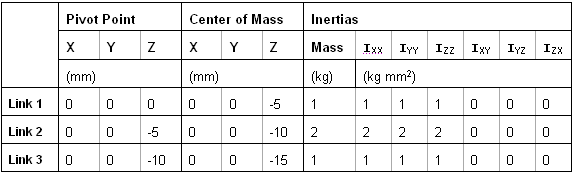
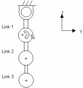
Apply this torque to estimate the natural frequencies of the triple pendulum
model shown in Figure 1:
Figure 1. Schematic representation of a triple pendulum in stable
equilibrium
Your analysis applies to a pendulum with any number of links or to more general
systems. Figure 2. Properties table for the triple pendulum
There are four MDL statements used in this
exercise:
Note: Refer
to the MotionView Reference Guide
(located in the HyperWorks Desktop Reference Guide) for the syntax
of the above MDL statements.
In a text editor, open an empty file.
Create the *DefineAnalysis() and
*EndDefine() block. You will add all other statements
between this block.
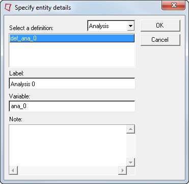
In the text editor, define an analysis with a variable name of
def_ana_0 and one argument j_att as an
attachment:
*DefineAnalysis(def_ana_0, j_att)
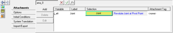
You can apply the torque between two bodies connected by a revolute joint, with
the origin of the joint taken as the point of application of the force. This
allows you to have only one attachment (the revolute joint). Create an
*Attachment() statement which defines
j_att as the attachment and Joint as the
entity type. Make sure that the variable name used in the statement is the same
as is used in the *DefineAnalysis() statement.
*Attachment(j_att, "Joint Attachment", Joint, "Select joint to apply
                        torque")
This allows you to only have one attachment; the revolute
joint.
Use the *ActionReactionForce() statement to define an
applied torque.
Remember: Reference the correct properties of the attachment joint
to reach the bodies involved in the joint. Refer to the description of the
dot separator in MDL. You can access properties of an entity by using the
dot separator. For example, bodies attached to the revolute joint can be
accessed as: <joint variable name>.b1 and as
<joint variable name>.b2
For the *ActionReactionForce() statement, define a
variable name of force_1.
Define the force type as ROT (rotational).
Define body 1 as j_att.b1 (attachment joint body
1).
Define body 2 as j_att.b2 (attachment joint body
2).
Define the force application point as j_att_i.origin
(the attachment joint origin).
Define the reference frame as Global_Frame
(global).
 (file browser) and select
analysis.mdl. Then click
Import.
(file browser) and select
analysis.mdl. Then click
Import.
 .
.
 (Run) panel
button.
(Run) panel
button.
 (Start/Pause Animation) button
to view the animation.
(Start/Pause Animation) button
to view the animation.