MV-1000: Interactive Model Building and Simulation
In this tutorial, you will learn how to create a model of a four-bar trunk lid
mechanism interactively through the MotionView graphical user
interface, perform a kinematic analysis on the model using MotionSolve, and post-process the MotionSolve results in the animation and plot windows.
A brief overview of Multi Body Dynamics (MBD) is provided below.
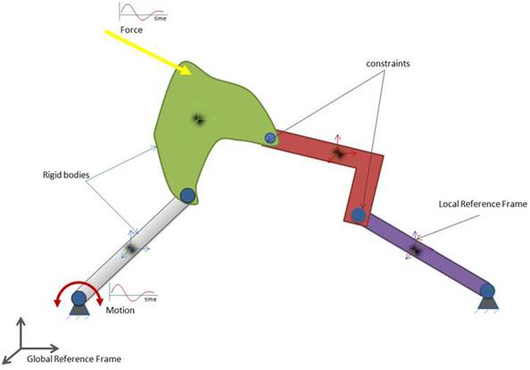
Multi Body Dynamics (MBD)
MBD is defined as the “study of dynamics of a system of interconnected
bodies”. A mechanism (MBD system) constitutes a set of links (bodies)
connected (constrained) with each other to perform a specified action
under application of force or motion. The motion of mechanisms is
defined by its kinematic behavior. The dynamic behavior of a mechanism
results from the equilibrium of applied forces and the rate of the
change of momentum.
MBD Modeling
A classical MBD formulation uses a rigid body modeling
approach to model a mechanism. A rigid body is defined as a body in
which deformation is negligible. In general, to solve an MBD problem,
the solver requires following information:
Rigid body inertia and location.
Connections – type, bodies involved, location, and
orientation.
Forces and motions – bodies involved, location, orientation, and
value.
MotionView facilitates quick and easy ways of
modeling items, such as a system, through graphical visualization. Figure 1.
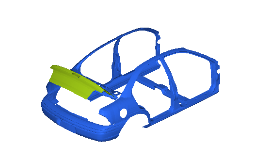
Trunk-Lid Model
The trunk-lid shown in the image below uses a four-bar mechanism for its
opening and closing motions. Figure 2. Car Trunk-Lid Mechanism
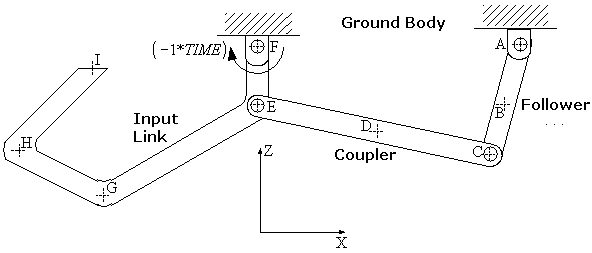
Below is a schematic diagram of the mechanism: Figure 3.
The four links (bodies) in a four-bar mechanism are: Ground Body,
Follower, Coupler, and Input Link. In this example, the Ground Body is
the car body and Input Link is the trunk-lid body. The remaining two
bodies (Follower and Coupler) form the part of the mechanism used to aid
the opening and closing of car trunk-lid.
The following entities are
needed to build this model:
Points
Bodies
Constraints (Joints)
Graphics
Input (Motion or Force)
Output
Create Points
In this step you will learn how to create points for your model.
From the mbd_modeling\interactive
folder, copy trunk.hm and trunklid.hm to the
<working directory>.
Start a new MotionView Session.
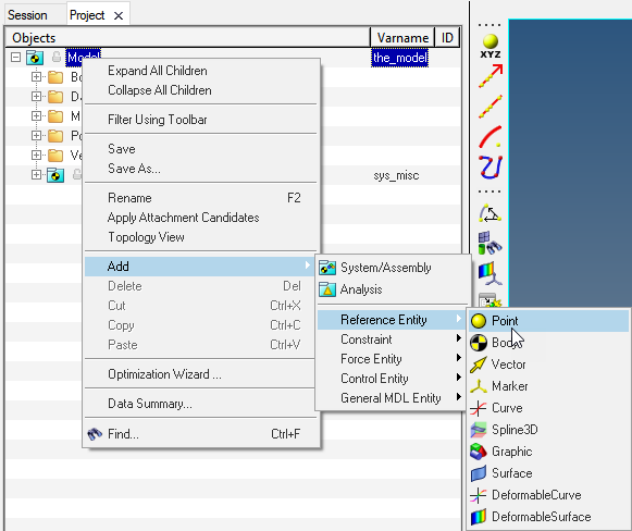
Add a point using one of the following methods:
From the Project Browser, right-click on
Model and select Add > Reference Entity > Point from the context menu. Figure 4.
On the Reference Entity toolbar, right-click on the (Points) icon.
The Add Point or PointPair dialog will be
displayed.
Note: Other entities like Bodies, Markers, and so on can also be
created using either of the methods listed above (Project Browser or toolbar).
For Label, enter Point A.
For Variable, enter p_a.
Figure 5.
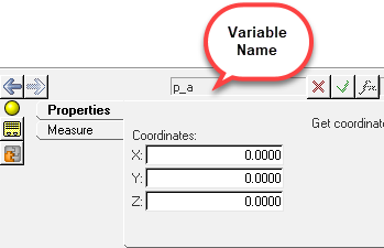
The label allows you to identify an entity in the modeling window, while the variable name is used by MotionView to uniquely identify an entity.
Note: When
using the Add "Entity" dialog for any entity, you can
use the label and variable defaults. However, as a best modeling practice,
it is recommended that you provide meaningful labels and variables for easy
identification of the entities. For this exercise, please follow the
prescribed naming conventions.
Click OK.
The Points panel is displayed. Point A is
highlighted in the Points list of the Project Browser. Figure 6. Points Panel - Properties Tab
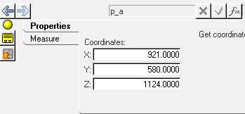
Enter the values for the X, Y,
and Z coordinates for point A.
Figure 7.
Create multiple points.
To create points B through I, repeat steps 2 through 4 and click
Apply.
Remember: Substitute B, C, and so on for A when entering
the label and variable names in the Add Point
or PointPair dialog. Clicking the Apply button allows you to continue to add
points without exiting the Add "Entity"
dialog.
After keying in the label and variable name for Point I, click
OK to close
the dialog.
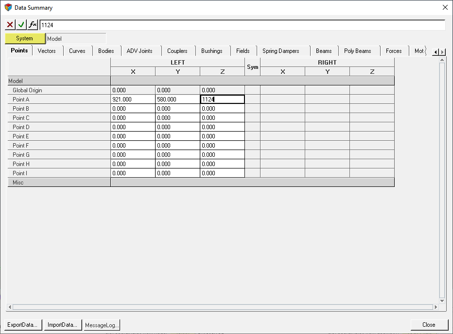
In the Points panel, click the Data Summary...
button.
The Data Summary dialog shows the table of
points and you can enter all the coordinates in this table. Figure 8.
Table 1.
Point
Location
Label
Variable
X
Y
Z
Point A
p_a
921
580
1124
Point B
p_b
918
580
1114
Point C
p_c
918
580
1104
Point D
p_d
915
580
1106
Point E
p_e
878
580
1108
Point F
p_f
878
580
1118
Point G
p_g
830
580
1080
Point H
p_h
790
580
1088
Point I
p_i
825
580
1109
Since the Y value for all the points are the same, you can
parameterize the value for points B through I to the value of Point A.
This process is explained in the next step.
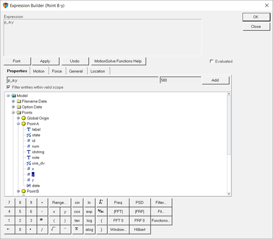
Parameterize the value for points B through I to the value of Point A.
Select the Y coordinate field along Point
B.
Click on the button to invoke the Expression
Builder.
Select the Y value of Point A.
Figure 9.
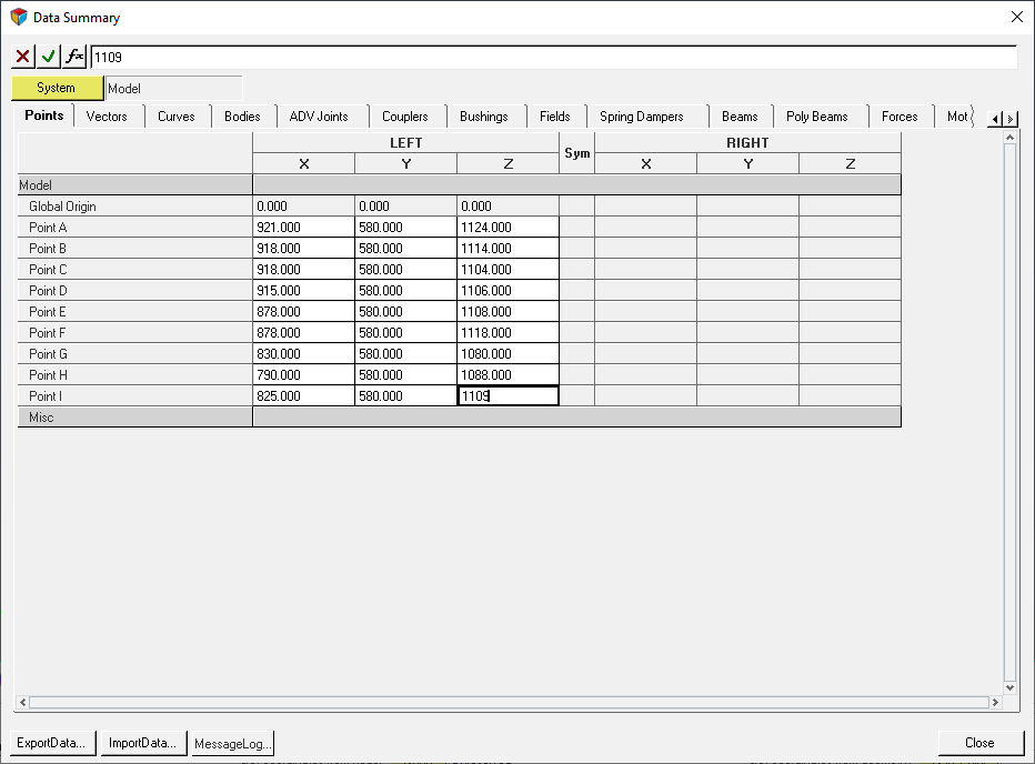
Copy the expression and paste into the Y coordinate
field of the remaining points.
Enter the X and Z coordinates as listed in the table above.
Note: On the keyboard, press Enter to move on to the next field in the table. Figure 10.
Click Close.
On the Standard Views toolbar, change the view to left by clicking the (XZ Left Plane View) icon.
Create Bodies
In this step, you will create the Input Link, Coupler, and Follower rigid-body links
in the mechanism.
The mechanism consists of four rigid-body links: Ground (car body), Input Link,
Coupler, and Follower. Ground Body is available by default when a new MotionSolve client is invoked, hence creating the Ground Body separately is
not required.
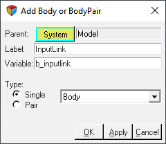
On the Reference Entity toolbar, click the (Bodies) icon.
In the Add Body or BodyPair dialog, Specify the label as
InputLink and the variable name as
b_inputlink.
Figure 11.
Click OK.
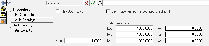
Enter the values for mass and inertia.
Click the Properties tab.
Enter the following values:
Mass=1
Ixx, Iyy, Izz= 1000, Ixy, Ixz,
Iyz=0
Figure 12.
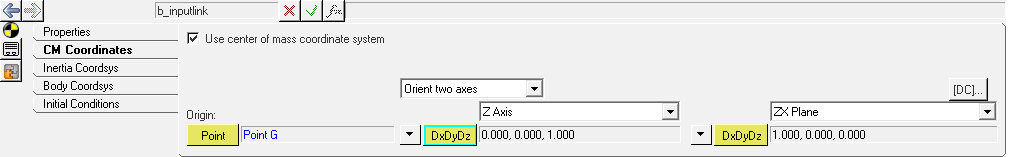
Click the CM Coordinates tab to specify the
location of the center of mass of the body.
Select the Use center of mass coordinate system check
box.
Under Origin, click the
(Point collector).
A cyan border will appear around the collector to indicate it is now
active for selection.
Select Point G.
Click again to launch the Select a
Point dialog.
Select Point G from the Model Tree.
Figure 13.
Click OK.
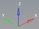
Figure 14.
Retain the default orientation scheme (orient two axes) and accept the
default values for .
Note: This method for selecting a point can also be applied to other entities
such as: body, joint, and so on. For selecting the Ground Body or the Global
Origin, you can click on the triad representing the Global Coordinate System
on the screen .
Tip: You can also select Point G from the modeling window. Hold down the left mouse button and
highlight Point G. Release the button to select
it.
Figure 15.
Repeat step 1 through 7 to create the remaining links with the variable names listed
in Table 2.
Table 2.
Label
Variable Name
Follower
b_follower
Coupler
b_coupler
Specify the mass and inertia for these links.
Mass= 1
Ixx, Iyy, Izz= 1000
Ixy, Ixz, Iyz=0
Specify points B and D as the
origin of the center of mass marker for Follower and Coupler,
respectively.
Retain the default orientation (Global coordinate system) for the CM
marker.
Create Revolute Joints
In this task you will learn how to create the joints necessary for this
model.
The mechanism consists of revolute joints at four points: A, C, E, and F. The axis
of revolution is parallel to the global Y axis.
Add a Joint in one of the following ways:
From the Project Browser, right-click on
Model. From the context menu, select Add > Constraint > Joint.
Click the (Joints) icon.
The Add Joint or JointPair dialog will display. Figure 16.
Specify the label as Follower-Ground and variable names
as j_follower_ground for the new joint.
Under Type, select Revolute Joint from the drop-down
menu.
Click OK.
The Joints panel will be displayed. The new joint
you added will be highlighted in the Model Tree in the
Project Browser.
Under the Connectivity tab, double click (first Body
collector).
The Select a Body dialog is displayed.
From the Model Tree, select
Bodies from the left-hand column and
Follower from the right-hand column.
Figure 17.
Click OK.
Notice that in the Joints panel the Follower Body is selected for and the cyan border moves to
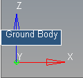
Click in the modeling window. With the left mouse
button pressed, move the cursor to the global XYZ triad.
Release the left mouse button when Ground Body is displayed in the modeling window.
Figure 18.
Under Origin, double click the
collector.
the Select a Point dialog will
display.
Select Point A as the joint origin.
Click OK.
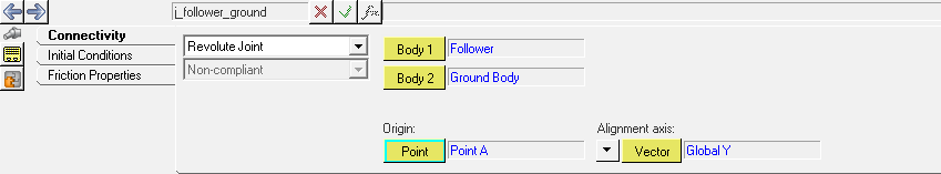
To specify an axis of rotation, under Alignment Axis, click the downward
pointing arrow next to Point and select Vector.
Specify the Global Y axis vector as the axis of rotation
of the revolute joint.
Figure 19.
Repeat steps 1
through 14 to
create the three remaining revolute joints: points C, E, and F. Use the
specifications shown in Table 3.
Table 3. Revolute joint information
Revolute Joint Label
Variable Name
Body 1
Body 2
Point
Vector
Follower-Ground
j_follower_ground
Follower
Ground
A
Global Y
Follower-Coupler
j_follower_coupler
Follower
Coupler
C
Global Y
Coupler-Input
j_coupler_input
Coupler
Input Link
E
Global Y
Input-Ground
j_input_ground
Input Link
Ground
F
Global Y
Specify a Motion for the Mechanism
In this step you will learn how to add motion to your mechanism model.
The input for this model will be in the form of a Motion. A Motion can be specified
as Linear, Expression, Spline3D, or Curve. In this step, you will specify a Motion using
an Expression.
Bring up the Add Motion or MotionPair dialog in one of the
following ways:
From the Project Browser, right-click on
Model and select Add > Constraint > Motion from the context menu.
On the Constraint toolbar, right-click on the (Motion) icon.
Specify the label as Motion_Expression and the variable
name as mot_expr.
Click OK.
The Motion panel is displayed. The new motion is
highlighted in the model tree in the Project Browser.
From the Connectivity tab, double click on the (Joint
collector).
The Select a Joint dialog is
displayed.
From the Model Tree, select the revolute joint at
Point F (Input Ground) that you created in the
previous step.
Figure 20.
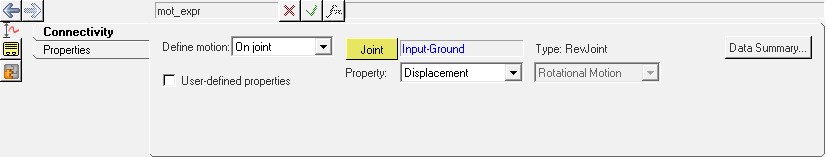
Click OK.
The Motion panel will be displayed. Figure 21.
From the Properties tab, under Define by, click on the gray arrow and select
Expression.
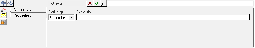
Click in the Expression field.
The Expression Builder is now activated. Figure 22.
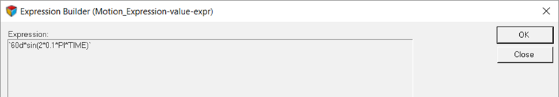
Click on the button to open the Expression Builder and enter
following expression between the back quotes
`60d*sin(2*0.1*PI*TIME)`.
Figure 23.
The expression is a SIN function with an amplitude of 60 degrees and
frequency of 0.1 Hz. With this expression the trunk lid is opened to an angle of
60 degrees and back in a total time period of 5 seconds.
Click OK.
Note: This method of creating an expression can also be used for specifying
nonlinear properties of other entities like Force, Spring Damper, Bushing,
and so on.
Create Outputs
In this step, you will add a displacement output between two bodies using the default
entities. You will also add another output to record the displacement of a particular point
G on the input link relative to the global frame based on Expressions.
You can create outputs using bodies, points and markers. You can also directly
request force, bushing, and spring-damper entity outputs. Another way to create outputs
is to create math expressions dependent on any of the above mentioned entities.
Open the Add Output dialog in one of the following ways:
From the Project Browser, right-click on
Model and select Add > General MDL Entity > Output from the context menu.
On the General MDL toolbar, right-click the (Outputs) icon.
Specify the label as Input Link Displacement and the
variable name as o_disp for the new output.
Figure 24.
Click OK.
Create a Displacement output between two points on two
bodies.
For Body 1 and Body 2, select Input Link and
Ground Body, respectively.
For Pt on Body 1 and Pt on Body 2, select point
I and the Global Origin point
respectively.
Record the displacement on Both points, one
relative to the other.
Figure 25.
Add one more output with the label as Input Link CM
Displacement and the variable name as
o_cm_disp.
Calculate the X displacement between the CM markers Input Link and the global
origin.
From the drop-down menu, select
Expressions.
Click in the F2 field.
This activates the button.
To display the Expression Builder dialog, Click on the button.
Clear the value 0 from the back-quotes.
From the Motion tab, click DX.
Place the cursor inside the curly-brackets {} after DX.
From the Properties tab, expand the following trees:
Bodies/Input Link/Marker CM.
Select idstring.
Figure 26.
Click Add to populate the expression.
Add a comma to separate the next expression.
Add a pair of curly brackets "{}".
Place the cursor inside the added brackets.
From the Properties tab, expand the following items in the tree:
Markers/Global Frame.
Select idstring.
Click Add to populate the expression.
Click OK
To check for errors, go to the Tools menu and select
Check Model.
Any errors in your model topology are listed in the Message
Log. Figure 27.
Attention: The ID numbers appearing in the expressions may
vary with the images shown.
Note: The DX function measures the
distance between Input Link’s CM (center of mass) marker and marker
representing the Global Frame in the X direction of the Global Frame. Refer
to the MotionSolve Reference Guide for more
details regarding the syntax and usage of this function.
The back quotes
in the expression are used so that the MDL math parser evaluates the
expression. Entity properties like idstring, value, etc. get evaluated
when they are placed inside curly braces {}, otherwise they are
understood as plain text. Refer to the Appendix to learn more about various
kinds of expressions and form of evaluation adopted by MotionSolve.
Add Graphic Primitives
In this step you will add graphics for visualization of the mechanism.
At this stage your trunk lid model does not contain any graphics, and the entities
created in previous steps are represented only by implicit graphics (which are not
available in solver deck or results file). Figure 28. Trunk-lid with only implicit graphicsMotionView graphics can be broadly categorized into
three types: implicit, explicit, and external graphics.
Implicit Graphics
The small icons that you see in the MotionView
interface when you create entities like points, bodies, joints, and so on
are called implicit graphics. These are provided only for guidance during
the model building process and are not visible when animating
simulations.
Explicit Graphics
These graphics are represented in form of a tessellation, are written to the
solver deck and subsequently available in the results. Explicit graphics are
of two types.
Primitive Graphics
These graphics help in better visualization of the model and are also
visible in the animation. The various types of Primitive Graphics in
MotionView are Cylinder, Box, Sphere, and so
on.
External Graphics
You can import in various CAD formats or HyperMesh files into MotionView. The ‘Import CAD or FE using HyperMesh..’
utility in MotionView can be used to convert a
CAD model or a HyperMesh model to
h3d graphic format which can be imported into
MotionView. One can also import
.g, ADAMS View .shl and
wavefront .obj files directly into MotionView.
MotionView allows you to turn on and off implicit
graphics for some of the commonly used modeling entities
Turn on implicit graphics.
From the Model main menu, select Implicit
Graphics...
Turn on the Visible check box.
Figure 29.
Note: Implicit graphics of Individual entities can be turned on or off
by using the Visible check box for each entity.
Click Close.
Note: The state of the implicit graphics (whether on or off) is not
saved in your model (.mdl) or session
(.mvw) files. MotionView uses its default settings when:
You create a new model in another model window.
You start a new session.
You load an existing
.mdl/.mvw file
into a new MotionView
session.
To visualize the four-bar mechanism, you need to add
explicit graphics to the model. In this step, you will add
cylinder graphics for Follower, Coupler, and Input
Links.
To add explicit graphics to your model, open the Add Cylinder or
CylinderPair dialog in one of the following ways:
From the Project Browser, right click on Model
and select Add > Reference Entity > Graphicfrom the context menu.
On the Reference Entity toolbar, right-click on the (Graphics) icon.
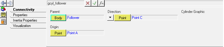
In the Add Cylinder or CylinderPair dialog, enter the
label as Follower Cylinder and the variable name as
gcyl_follower.
Figure 30.
Note: The name of the dialog changes with the graphic type. For example, the
dialog name changes to Add Box or BoxPair when the Box
graphic type is selected.
From the Type drop-down menu, select Cylinder.
Click OK.
In the Connectivity tab, double-click on the (Body button) below
Parent.
Select the Follower from the Select a Body list and
click OK.
This assigns the graphics to the parent body.
To select the origin point of the cylinder, click
below Origin.
Pick Point A in the modeling window.
Click under Direction.
Select Point C for .
Figure 31.
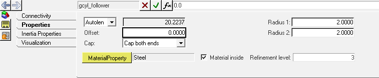
From the Properties tab, enter 2 in the Radius 1:
field.
Figure 32.
Note: The cylinder graphic can also be used to create a conical graphic. By
default, the Radius 2 field is parameterized with respect to Radius 1, such
that Radius 2 takes the same value of Radius 1. Specify different radii to
create a conical graphic.
For the remaining bodies in your model, follow steps 2 through 12 to create the
appropriate explicit graphics for other links. Use the specifics given in Table 4.
Table 4.
Label
Variable Name
Graphic type
Body
Origin
Direction
Radius
Follow Cylinder
gcyl_follower
Cylinder
Follower
Point A
Point C
2
Coupler Cylinder
gcyl_coupler
Cylinder
Coupler
Point C
Point E
2
Input Link Cylinder 1
gcyl_inputlink_1
Cylinder
Input Link
Point F
Point E
2
Input Link Cylinder 2
gcyl_inputlink_2
Cylinder
Input Link
Point E
Point G
2
Input Link Cylinder 3
gcyl_inputlink_3
Cylinder
Input Link
Point G
Point H
2
Input Link Cylinder 4
gcyl_inputlink_4
Cylinder
Input Link
Point H
Point J
2
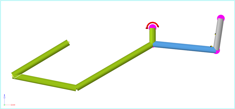
After the addition of cylinder graphics for all three links, the Model
will look as shown in Figure 33: Figure 33.
Add External Graphics and Convert a HyperMesh File to an H3D
File.
In this step you will use this conversion utility to convert a HyperMesh file of a car trunk lid into the H3D format.
MotionView has a conversion utility that allows you to
generate detailed graphics for an MDL model using HyperMesh,
Catia, IGES, STL, VDAFS, ProE, or Unigraphics source files. MotionView uses HyperMesh to perform
the conversion.
From the Tools menu, select Import CAD or FE using HyperMesh.
From the Import CAD or FE using HyperMesh dialog, activate the
Import CAD or Finite Element Model Only radio
button.
From the Input File option drop-down menu, select HyperMesh.
Click the button next to Input File and select
trunklid.hm, located in your <working
directory>, as your input file.
The Output Graphic File will be automatically
populated with the trunklid_graphic.h3d file from the
<working directory>.
Click OK to begin the import
process.
Figure 34.
The Import CAD or FE using HyperMesh utility
runs HyperMesh in the background to translate the
HyperMesh file into an H3D file. When the import
is complete the Message Log appears with the message
"Translating/Importing the file succeeded!"
Note: The H3D file format is a
neutral format in HyperWorks. It finds wide
usage such as graphics and result files. The graphic information is
generally stored in a tessellated form.
Clear the Message Log.
Use steps 1
through 6 to
import the trunk graphics by converting the trunk.hm file
to trunk.h3d.
Attach H3D Object to the Input Link and Ground Bodies
In this step, you will attach the trunk lid H3D object to the input link and the
trunk H3D object to Ground.
On the Reference Entity toolbar, click (Graphics).
Select g_trunklid_graphic from the modeling window.
In the Connectivity tab, double click the
(Body collector).
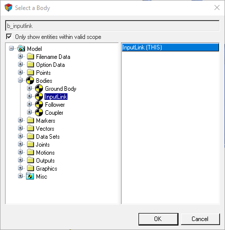
From the Select a Body dialog, click Input Link.
Figure 35.
Click OK.
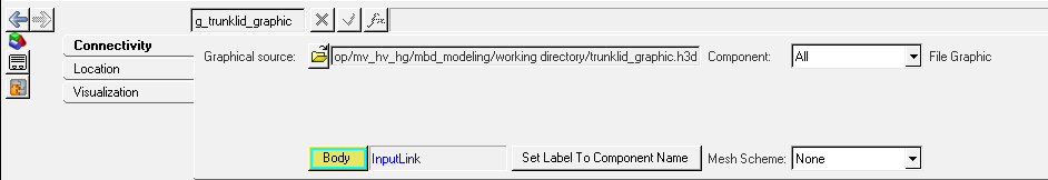
This will display the Graphics panel. Figure 36.
Note: Observe the change in the trunk lid graphic color to the Input Link
body color.
Select the newly created g_trunk_graphic from the Project Browser and set the as
Ground Body.
On the Standard toolbar, click the Save Model icon
.
If the model is new you will be prompted to input the name of the model,
otherwise the model will be saved in the working directory with the existing
name.
Note: Existing models can be saved to another file using the Save As > Model option located in the File menu.
From the Save As Model dialog, browse to your working
directory and specify the file name as
trunklid_mechanism.mdl.
Figure 37.
Click Save.
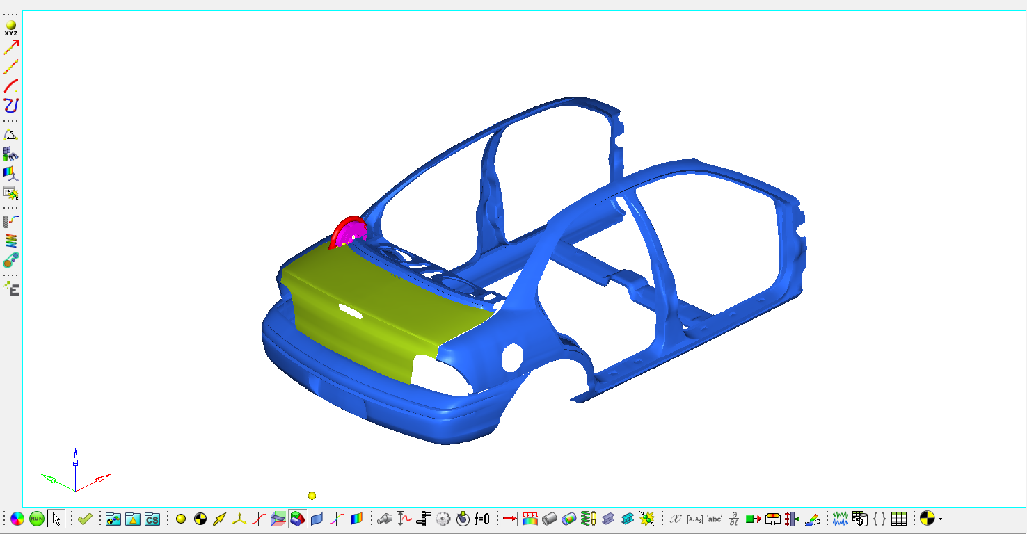
Figure 38. Trunk-lid mechanism
Solve the Model with MotionSolve
In this step, you will use MotionSolve to perform a
kinematic simulation of the mechanism for a simulation time of 5 seconds, with a step size
of 0.01 second.
MotionSolve can be used to perform kinematic, static,
quasi-static, and dynamic analyses of multi-body mechanical systems. The input file for
MotionSolve is an XML file called MotionSolve XML. The solution in MotionSolve can be executed from MotionSolve.
On the General Actions toolbar, click the (Run) icon.
On the Model Check toolbar, click on the (Check model) button to check the model for errors.
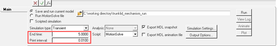
From the Main tab of the Run panel, specify Transient as
the Simulation type.
Specify the name for the XML file as
trunklid_mechanism_run.xml.
MotionView uses the base name of your XML file for
other result files generated by MotionSolve. See the
MotionView User’s Guide for
details about the different result file types.
Activate the Export MDL snapshot check box (if it is not
already active).
This will save the model at the stage in which the Run is
executed.
Specify an End time of 5 for your simulation and a Print
interval of 0.01
Figure 39.
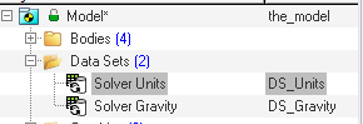
Note: The time unit is based on the time unit chosen (default is Seconds).
You can access the Solver Units and Gravity Data Sets from the Project Browser. Figure 40.
.
To solve the model with MotionSolve, click the
Run button.
Note: Check the Message Log for more information.
Upon clicking Run, MotionSolve is invoked and solves the model. The
Solver View window appears which shows the progress of
the solution along with messages from the solver (Run log). This log is also
written to a file with the extension .log to the solver
file base name.
Review the window for solution information and be sure to watch for any
warnings/errors.
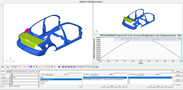
View Animation and Plot Results on One Page
In this step you will learn to view your animation and plot result on the same
page.
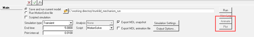
Once the run is successfully complete, both the Animate and Plot buttons are
active. Figure 41.
Click the Animate button.
This opens HyperView in another window and
loads the animation in that window.
On the toolbar, click the icon to start the animation.
Note: You can click the button again to stop/pause the
animation.
Return to the MotionView window.
Click the Plot button.
This opens HyperGraph and loads the results
file in a new window.
REQ/70000000 InputLink from Ground Body (Input Link
Displacement)
Y Component
DM (Magnitude)
Click Apply.
This plots the magnitude of the displacement of Point I relative to the
Global Origin. Figure 42. Session with model, plot, and animation
Save Your Work as a Session File
Here, you will learn to save your model as a session file.
From the File menu, select Save As > Session File.
Specify the file name as trunklid_mechanism for your
session.
Click Save.
Your work is saved as trunklid_mechanism.mvw
session file.
Appendix
Evaluating Expressions in MotionView.
Table 6.
Math Parser
A MotionView parser that
evaluates a MotionView expression as real/integer/string
for a field as appropriate
Real
This type of field can contain a real number or the parametric expression that
should evaluate to a real number. This type of field is found in Points, Bodies,
Force – Linear. Note that only the value of the expression as evaluated goes into
the solver deck and not the parametric equation.
Example: p_a.x,
b_0.mass
String
This type of field can contain a string or a parametric expression that should
evaluate to a string. This type of field is found in entity such as DataSets with
strings as Datamember, SolverString etc. As in case of Linear field, only the value
of the expression as evaluated goes into the solver deck and not the parametric
expression.
Example: b_inputlink.label
Integer
This type of field can contain an integer or a parametric expression that
evaluates to an integer. This type of field is found such as DataSets with an
integer as Datamember. Even in this case, only the value of the expression as
evaluated goes into the solver deck and not the parametric equation.
Table 7.
Templex Parser
A math program available in HyperWorks that can perform more complex programming than the
math parser, other than evaluating a MotionView
expression. The following type of fields in MotionView
are evaluated by the templex parser that evaluates a parameterized
expression:
Expressions
This type of field is different than the three listed above because it can
contain a combination of text and parametric expression. It is generally used to
define a solver function (or a function that is recognized by the solver). This type
of expression is embedded within back quotes ( ` ` ) and any
parametric reference is provided within curly braces {}. The presence of back quotes
suggests the math parser to pass the expression through Templex. Templexevaluates any
expression within curly braces while retaining the other text as is. For example in
the expression `
DX({b_inputlink.cm.idstring},{Global_Frame.idstring})`, the templex
evaluates the ID (as a string) of the cm of the Input link body (b_
inputlink) and that of marker Global Frame while retaining “DX” as is.
These fields are available in entity panels such as: Bushings, Motions, Forces with
properties that toggle to Expression, Independent variable for a curve input in
these entities, and Outputs of the type Expression.
 (Points) icon.
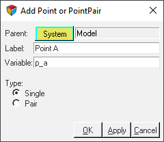
 button to invoke the Expression
Builder.
button to invoke the Expression
Builder.
 (XZ Left Plane View) icon.
 (Bodies) icon.
 (Point collector).
A cyan border will appear around the collector to indicate it is now active for selection.
(Point collector).
A cyan border will appear around the collector to indicate it is now active for selection.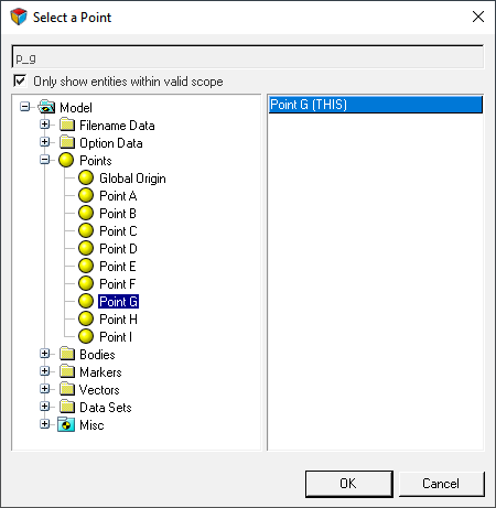
 .
.
 .Tip: You can also select Point G from the modeling window. Hold down the left mouse button and highlight Point G. Release the button to select it.
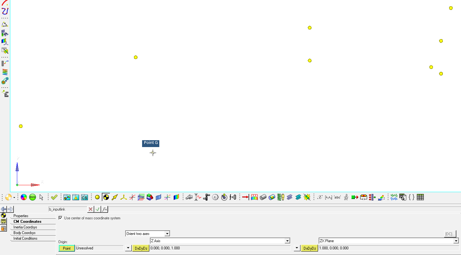
 (Joints) icon.
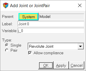
 (first Body
collector).
The Select a Body dialog is displayed.
(first Body
collector).
The Select a Body dialog is displayed.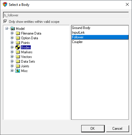

 (Motion) icon.
 (Joint
collector).
The Select a Joint dialog is displayed.
(Joint
collector).
The Select a Joint dialog is displayed.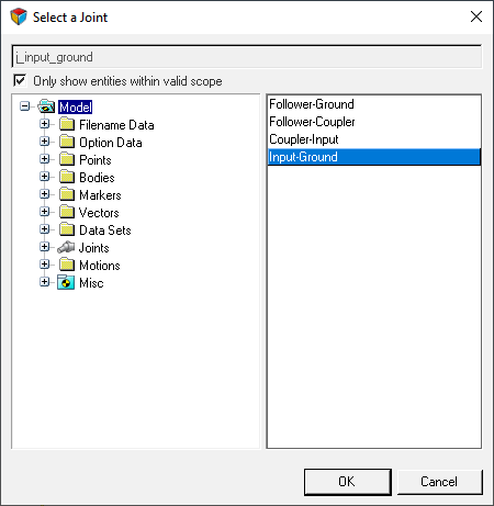
 (Outputs) icon.
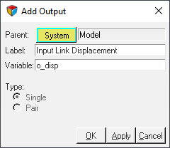
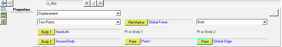
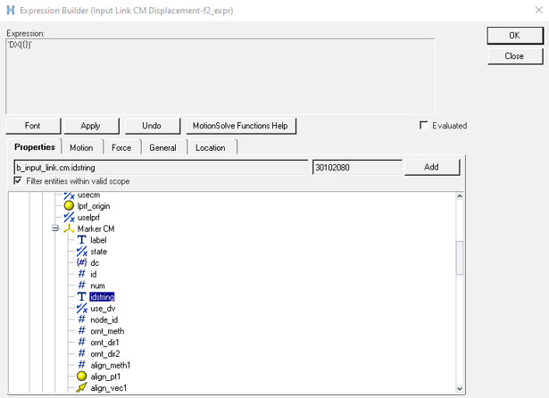
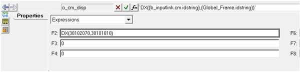
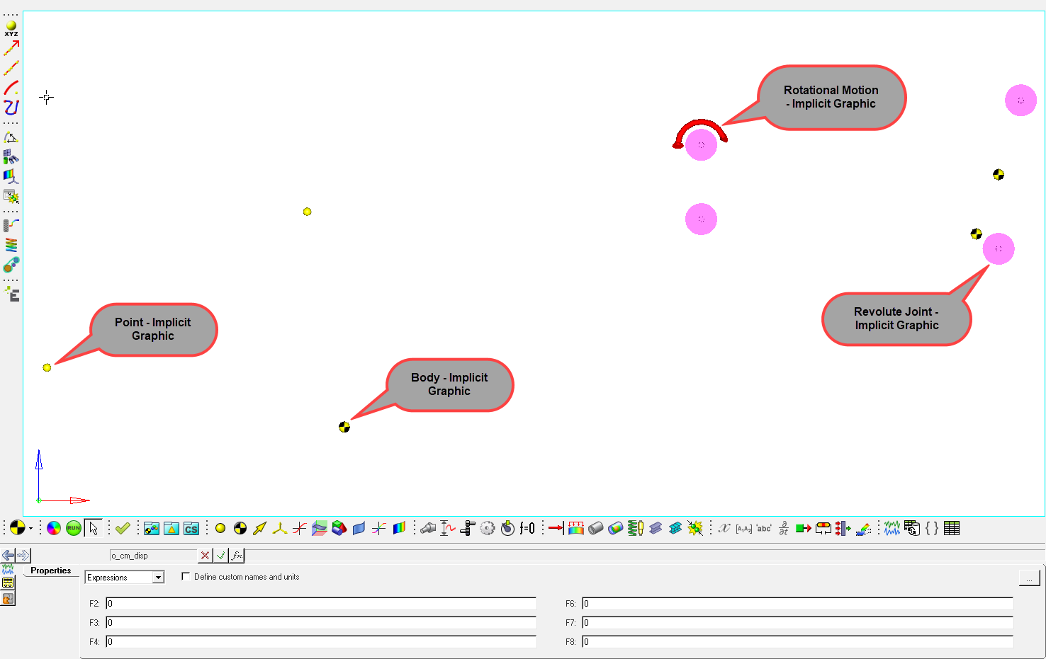
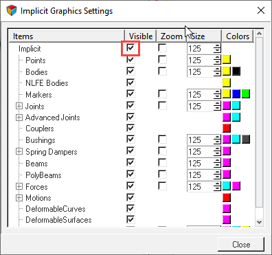 Figure 29. Note: Implicit graphics of Individual entities can be turned on or off by using the Visible check box for each entity.
 (Graphics) icon.
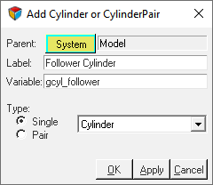
 (Body button) below
Parent.
(Body button) below
Parent.
 button next to Input File and select
trunklid.hm, located in your <working
directory>, as your input file.
The Output Graphic File will be automatically populated with the trunklid_graphic.h3d file from the <working directory>.
button next to Input File and select
trunklid.hm, located in your <working
directory>, as your input file.
The Output Graphic File will be automatically populated with the trunklid_graphic.h3d file from the <working directory>.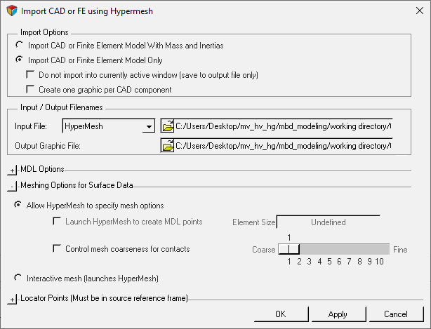
 .
If the model is new you will be prompted to input the name of the model, otherwise the model will be saved in the working directory with the existing name.Note: Existing models can be saved to another file using the option located in the File menu.
.
If the model is new you will be prompted to input the name of the model, otherwise the model will be saved in the working directory with the existing name.Note: Existing models can be saved to another file using the option located in the File menu.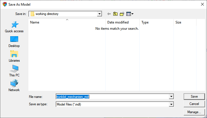
 (Run) icon.
 (Check model) button to check the model for errors.
 icon to start the animation.
Note: You can click the button again
icon to start the animation.
Note: You can click the button again to stop/pause the
animation.
to stop/pause the
animation.