MV-1035: Import CAD or FE into MotionView
In this tutorial, you will learn about an important modeling approach: Building an MBD model from CAD data.
- Import a CAD assembly into MotionView.
- Import a CSV file to create Points
- Create an MBD model using the imported data.
The Import CAD or FE utility in MotionView allows you to import CAD or FE assemblies. CAD formats include CATIA, Parasolid, Pro E, STEP, JT, SolidWorks and Unigraphics. FE formats include HyperMesh, OptiStruct, and Nastran.
CAD or FE assemblies can be imported into MotionView as graphics only to be associated with existing bodies, or as new bodies with calculated mass and inertia properties along with graphics.
- Component Mass
- Component Moments of Inertia
- Component Center of Gravity Location
- Component Graphics
The CAD import utility calls HyperMesh in the background to write out a graphic file (*.h3d) which holds the geometry information in a tessellated form. While importing CAD or FE to create new bodies with mass and inertia, the utility uses HyperMesh to calculate mass, inertia and CG location.
In the following exercise, you will import a CAD assembly into MotionView, simplify the model from a multibody analysis point of view, and define constraints, model inputs and model outputs.
Please copy all of the files from the mbd_modeling\automation\CAD folder into your <working directory>.
Load a CAD File in MotionView
In this step, the focus is on understanding the process of import and model simplification.
-
Launch a new MotionView session by clicking

-
From the menu bar, select
Or
Click Import Geometry
 , on the Standard toolbar.The Import CAD or FE dialog is displayed.
 -
Click
 to select the STEP file.
-
Click the plus button next to MDL Options and review the various options.
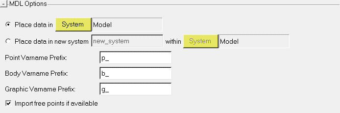
Figure 1.Note: The MDL Options allow for flexibility while importing. The CAD file can be imported either in an existing system/assembly or a new system can be created -
Review the options under Meshing Options for Surface Data.
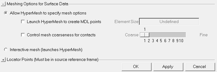
Figure 2.Note: This section helps control the size of mesh (or tessellation). When the MBD model being created is used to solve non-contact problems, use the default option under Allow HyperMesh to specify mesh options. The Launch HyperMesh to create MDL points option allows you to select nodes in HyperMesh which can be imported into MotionView as MDL points. This is not needed for this tutorial since you will be creating these additional points using a macro. For models that involves contacts, it is recommended to use Control mesh coarseness for contacts. The Interactive mesh (launches HyperMesh) option can be used to mesh the surfaces manually. This is particularly useful when a finer mesh may be needed, such as in case of contact problems, to obtain better results. -
Click the plus button next to Locator Points (must be in source reference
frame) and review the options.
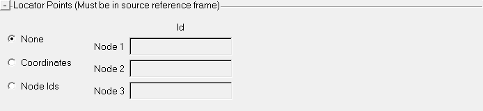
Figure 3.Note: The Locator Points options can be used in cases where the CAD model being imported is not in the same coordinate system as the MBD model in MotionView. This option gives you control to specify three nodes or coordinates on the source graphic which can then be used to orient using three points in MotionView after it's imported. This option is not needed for tutorial as the imported graphic is in the required position. -
Under Component, select Wheel_body1. In the Apply
density to selected components field, change the value of the density to
8.5e-7 and click Apply.
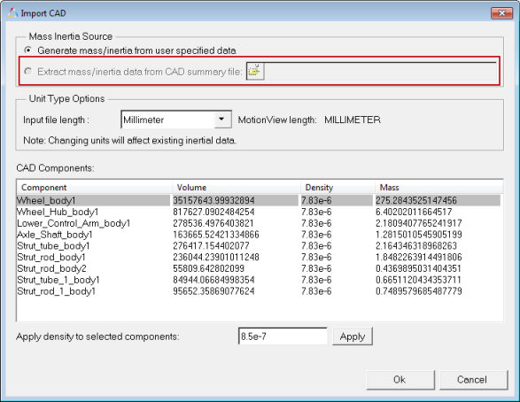
Figure 4. Import CAD Dialog
Consolidate and Rename the Suspension Assembly Bodies
-
In the Project Browser, select these bodies:
Strut_rod_1_body1,
Strut_rod_body1 and
Strut_rod_body2. Right-click to bring up the context
menu.
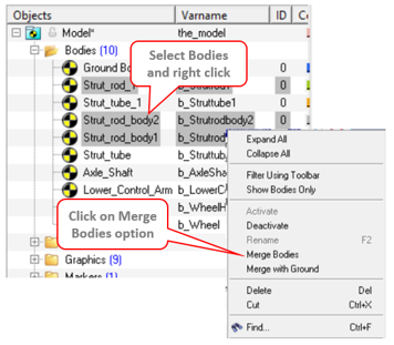
Figure 5. -
From the Merge Bodies dialog, enter
Strut_rod as the label and
b_Strut_rod as variable name. Click
OK.
The three selected bodies are deleted and replaced by a new body with the label and variable names as entered previously. The mass and inertia values of this body are equivalent to the effective mass and inertia of the bodies being replaced.
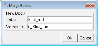
Figure 6. -
Save the model as front_susp.mdl.
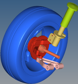
Figure 7.
- Mass and inertia of the newly created body upon Merge will be equal to the effective mass and inertias of the bodies being merged.
- A new CG point is created at the effective CG location of the bodies being merged.
- Pair bodies cannot be merged.
- The Merge option works only within same container (System/Assembly/Analysis). Merging bodies which belong to different container entities is not supported. The context menu item will not appear in these cases.
- If the bodies that are being merged are referred to in expressions, post Merge these expressions need to be corrected to point to the newly created body.
- Graphics that belong to bodies being merged are automatically resolved to the new body.
- Joints, bushings etc. that are associated with the bodies being merged if any, are automatically resolved to the new body.
Create Points
After creating the bodies, additional points are needed that will be used to specify joint locations and joint orientations. These points can be created using the macros available in the Macros menu.
-
From the Macros menu, select or click Create points using Coordinates
 .
.
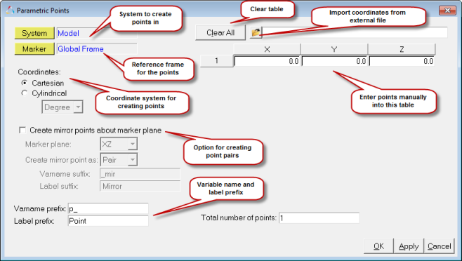
Figure 8. -
Click to load a point table file.
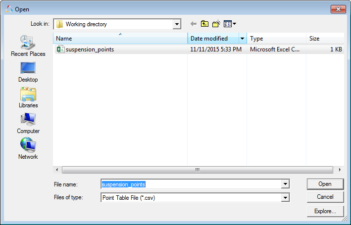
Figure 9. -
Click Open.
All the point coordinates in the CSV file are imported into the utility.
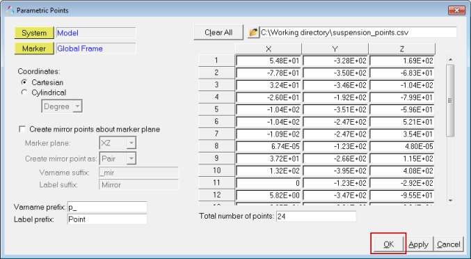
Figure 10. -
Click OK.
The points are added to the model. These extra points will be used for defining joints, orientations and other model inputs.Note: To use this macro import option, you have to create the *.csv file in the format shown below:
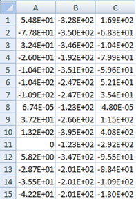
Figure 11.1st Column - X coordinates.
2nd Column - Y coordinates.
3rd Column - Z coordinates.
Create Joints and Spring Damper
In this step, you will add the joints to connect the bodies and a spring damper between Strut tube and Strut rod.
-
From the Project Browser, right-click
Model and select (or right-click Joints
 from the toolbar).
The Add Joint or JointPair dialog is displayed.
from the toolbar).
The Add Joint or JointPair dialog is displayed. -
Make the following selections:
- For Body1 of the joint, specify Wheel.
- For Body2, specify Wheel_Hub.
- For Origin, specify Point7. (Point around the Wheel center).
- For Axis, specify Point19. (Point around Axle Shaft center).
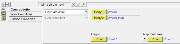
Figure 12. -
From the Project Browser, right-click
Model and select (or right-click
 icon from the toolbar).
Add a Jack to the Model
-
From the Project Browser, right-click
Model and select (or right-click Bodies
 from the toolbar).
-
From the Project Browser, right-click
Model and select (or right-click Graphics
 from the toolbar) to add a graphic.
-
From the Project Browser, right-click
Model and select (or right-click Joints
from the toolbar).
-
Save the model.
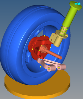
Figure 13. Front suspension
Specify Motion Inputs and Run the Model in MotionSolve
In this step, you will create a motion that is applied to the jack and solve the model.
-
From the Project Browser, right-click
Model and select (or right-click Motion
 from the toolbar) to add a motion.
-
Click Check Model
 . In the Message Log that is displayed, verify that
there are no warnings or errors. Clear the message log.
. In the Message Log that is displayed, verify that
there are no warnings or errors. Clear the message log.
-
Go to the Run panel
 .
.
-
Specify a name for the MotionSolve input XML file
by clicking Save and run current model
.