This tutorial shows how to create advanced functions in AcuFieldView to help quantify the extent of mixing in a static
mixer.
Prior to running this tutorial, copy the expanded polymer_mixing
directory from <AcuSolve installation
directory>\model_files\tutorials\AcuFieldView\AFV_tutorial_inputs.zip
to a working directory. See Tutorial Data for more information.
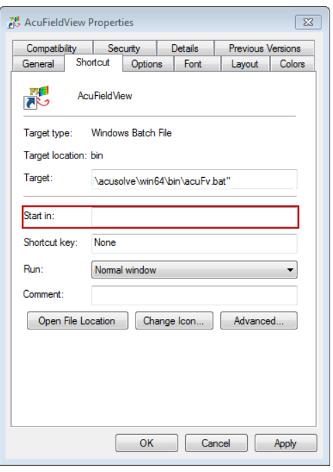
For Windows users, in order to take advantage of the restarts provided for this
tutorial, you will need to make sure that the properties for your AcuFieldView shortcut on the Start menu do not include a
Start in entry. To change that property, browse to the AcuFieldView shortcut on the Start menu, right-click, and
select Properties. The Start in field can be found on the
Shortcut tab in the AcuFieldView Properties dialog. Note
that this step is only necessary because the restart files use relative paths. Figure 1.
Solve the Case with AcuConsole and AcuSolve
Start
AcuConsole.
Open <your working
dir>\polymer_mixing\polymer_mixing.acs.
Generate a mesh.
Run
AcuSolve to calculate a solution.
Exit
AcuConsole.
Convert the Dataset to FieldView Unstructured Format (FV-UNS)
AcuFieldView's native format for reading data is known as
the FV-UNS format. This format has been optimized for file size and performance. When
using this format, data read times are reduced in comparison to reading the data
directly from the AcuSolve database. When the data will be
read multiple times, this format is preferred. This step explains how to perform the
conversion of AcuSolve results to FV-UNS format.
Open an AcuSolve Cmd Prompt or Linux terminal.
Change the directory to the location of the solved problem: <your
working dir>\polymer_mixing\.
Execute AcuTrans with the following command line
arguments.
acuTrans -out -to fieldview
Exit the command window or terminal when
AcuTrans completes the conversion.
Start AcuFieldView and Create Boundary Surfaces
Start
AcuFieldView.
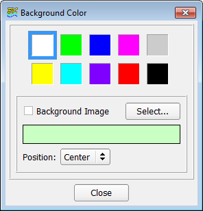
Click View > Background Color and select white.
Click Close.
Figure 2.
Click File > Data Input > AcuSolve [FV-UNS Export].
Click Read Grid or Combined Data.
Browse to the \polymer_mixing directory, select polymer_mixing_step000032.fv, and click Open.
Note: The file in your directory may have a slightly different step number. This
is expected due to processor and operating system differences.
In the Function Subset Selection panel, which opens up
with all of the functions selected by default, click
OK.
Close the
AcuSolve [FV-UNS Export] panel.
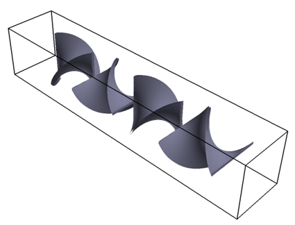
Click Bound to open the Boundary Surface panel.
Click Create.
Select OSF: Fin Walls in the BOUNDARY TYPES list to create a surface consisting of all of the blades and click OK.
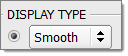
Change DISPLAY TYPE to Smooth shading.
Figure 3.
Click on the toolbar to open the Color Mixer panel.
Change the gray chip to Red, Green and Blue values of
130, 130 and
158.
Click Apply and click
Close.
In the Boundary Surface panel, BOUNDARY TYPES section, click OK.
Figure 4.
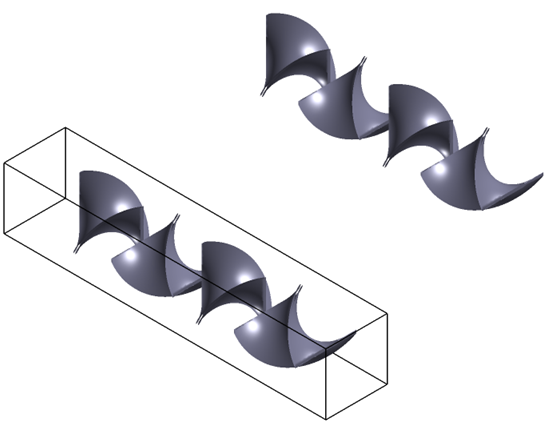
Click Create.
Select OSF: Fin Walls again and click OK.
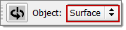
On the Transform Controls toolbar, change Object to Surface.
Figure 5.
Use the left mouse (M1) to translate the current boundary surface up and
right.
Click Viewer Options to open the Viewer Options panel.
Turn Perspective off and click Close.
Click View > Rendering Options.
Turn off everything except Boundary Surfaces and Streamlines.
Activate Presentation Quality.
Adjust the controls under LIGHTING INTENSITY and SHININESS and click
Refresh to see the effect of each change.
Click Default Light to restore the default LIGHTING
INTENSITY, reset Intensity and Highlight Size under SHININESS to
1 and 0.5, click
Refresh, and close the panel.
Figure 6.
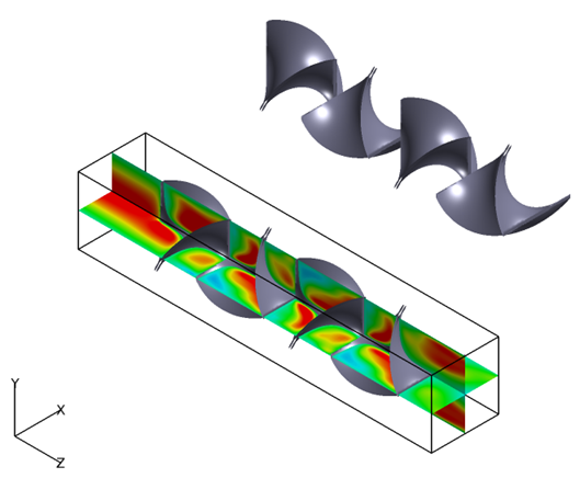
Click Coord
to open the Coordinate Surface panel.
Create an X Coordinate Surface.
Change DISPLAY TYPE to Smooth shading and COLORING to
Scalar.
Change the Scalar function to z-velocity and click Calculate.
Change the Colormap minimum value to -2.0 and maximum
value to 4.0.
Create a second coordinate surface at Y = 0.
Figure 7.
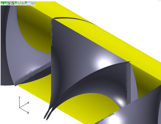
Visualize Back Flow
This step will help visualize the back flow resulting from the mixer blades.
On the Transform Controls toolbar, click
to turn the Outline off.
Turn off the Visibility of the coordinate surfaces and the surface transformed boundary surface (boundary surfaces ID 1 and ID 2).
On the Viewer toolbar, set Object to World.
Click Zoom
and use M1 (left mouse) to select an area to zoom into the third blade
element.
Create a boundary surface containing the BOUNDARY TYPES of OSF: Pipe Wall.
Turn on Visibility (if not already).
Change the Geometric COLORING to yellow.
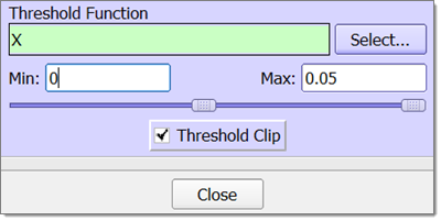
Click Select to change the Threshold Function.
On the Function Specification panel, select X and click Calculate.
Activate Threshold Clip, set the Min to
0 using the slider or by directly entering
0 in the Min field.
Figure 8. Figure 9.
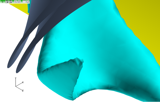
Click Iso to open the Iso-Surface panel.
Click Create.
Click Define Iso Function on the Iso-Surface Create panel.
Select z-velocity and click Calculate.
Change the Current value to -0.25 and the DISPLAY TYPE
from Constant to Smooth shading.
You will seed streamlines on this iso-surface.
Change the Geometric COLORING to light blue.
Figure 10.
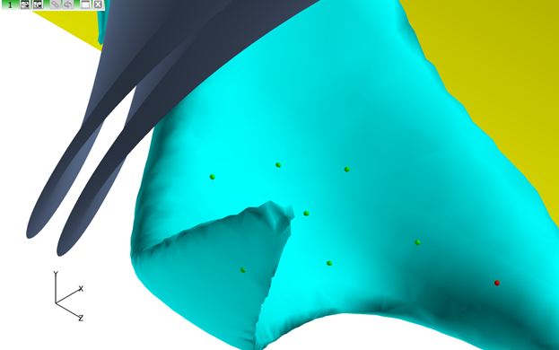
Click Stream or to open the Streamlines panel.
Click Create on the Rake tab.
Zoom with M1 further into the largest iso-surface region for easier seeding.
Use Ctrl + left mouse button (M1) to add eight seeds
(Ctrl click once per seed).
Figure 11.
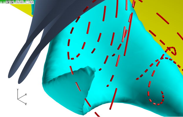
In the Calculation Parameters section, change Direction to
Both and the Step value to
6.
Click Calculate.
Change the DISPLAY TYPE to Filament, change Line Type to
Thick, change Geometric coloring to red and change
Div to 100.
Turn Show Seeds off.
Use M3 (right mouse) to zoom out.
Figure 12.
Note: The streamlines on your screen will differ from what is shown, based on
the placement of your seeds.
Turn on Animate to visualize the streamlines.
Click View > Minimum Time Between Frames and use the slider to slow the animation.
Turn off Animate for the next step.
View Axial Velocities
In this step, you will sample cross-sections of the static mixer to visualize axial
velocities. A restart is available to recreate this view.
Turn off the Visibility of the streamlines and the iso-surface.
Zoom out to view the entire dataset.
Create a coordinate surface at Z = -0.475.
Turn on Visibility, if needed.
The Scalar Function should still be z-velocity, the DISPLAY TYPE should be Smooth
shading, and the COLORING should be Scalar.
In the Colormap tab, change the colormap from Spectrum to
NASA-1.
Activate Filled Contour.
Change the Number of Contours to 64.
In the Legend tab on the Coordinate Surface panel, activate Show
Legend, change Decimal Places to 2, change the number
of Labels to 5 and clear the Subtitle field.
Hold down Shift, position the mouse over the legend, then
left-click and drag to position the legend.
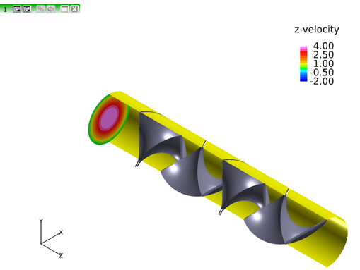
Figure 13.
On the Surface tab of the Coordinate Surface panel, click Create again to create an identical surface.
This new surface will be moved and oriented separately from the rest of the
model.
On the Viewer toolbar, set Object to Surface.
Move the surface up.
On the Viewer toolbar, click to activate the locked transformation controls.
Use the icons on the Viewer toolbar to rotate the surface to the orientation illustrated.
Figure 14.
There are two modes of operation of the locked transformations controls. When the mouse icon has
a light background , you can click the toolbar icons to transform
the surface. When the mouse icon has a darker background , you can perform transformation by clicking a pair of toolbar
icons and then using the right mouse to transform the surface.
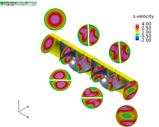
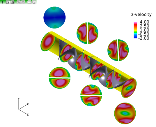
Figure 15.
Create five more pairs of surfaces at Z values of -0.35,
-0.25, -0.15, -0.05
and 0.05.
Move and rotate one of each surface pair, as illustrated.
Click on the Viewer toolbar to toggle to Locked
Transforms control and move the coordinate surface up.
Figure 16.
Change the Scalar Display of the Cross Sections
This step shows how to create similar images of several other useful flow properties.
Defining these flow properties involves using the function calculator to define the
equations and variables needed. The formula needed can be found in a formula restart
file that is provided for this tutorial.
Double click on the coordinate surface above the upstream end of the mixer.
Click File > Open Restart > Formula to open the OPEN RESTART: Formula
panel.
In the polymer_mixing\restart
directory, select
polymer.frm and click
Open.
Click the icon.
Click Scalar on the
Function Selection panel.
Scroll down in the list, select
shear, and click
Calculate.
Close the Function Specification panel.
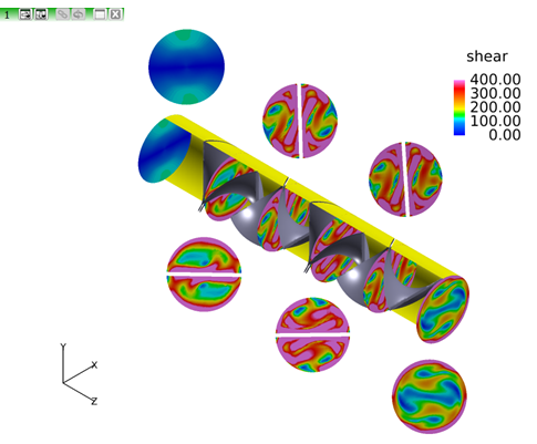
On the Colormap tab of the Coordinate Surface
panel, change the minimum and maximum SCALAR
COLORING values to 0.0 and
400.
Figure 17.
Steps 2-6 above display the shear function on
the current surface. Note that the legend title
reflects the scalar values for the surface with
the visible legend.
Click Tools > Unify to force all of the coordinate
surfaces in the dataset to acquire the same
attributes as the current surface.
This will also update the legend, as the
surface it belongs to will inherit shear as the Scalar Function. Unify only applies
changes to all surfaces of the same type as the currently active surface. Figure 18.
Double click the legend to open the Coordinate Surface panel with the ID for the surface with the visible legend.
Click the icon.
Click Scalar on the
Function Selection panel.
Scroll down in the list (if needed), select
lambda, and click
Calculate.
Close the Function Specification panel.
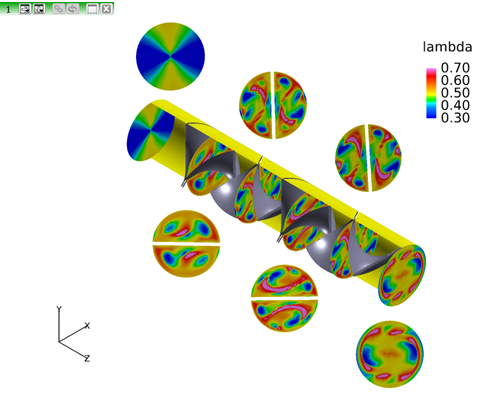
On the Colormap tab of the Coordinate Surface
panel, adjust the min/max SCALAR COLORING to
0.30 and
0.70.
At this point, the legend should now be
updated to show the contours for lambda.
Click Tools > Unify to apply lambda as the scalar
function for all coordinate surfaces.
The mixing parameter is interpreted as
follows:
0.0 = simple rotation
0.5 =
simple shear
1.0 = elongation
Figure 19.
Integrate Concentration Variance of Each Cross Section
This step will be similar to the last step in that you will change the scalar function
being displayed on the coordinate surface.
Double click the legend to open the Coordinate Surface panel for the surface with the visible legend.
Click the
icon.
Tip: As an alternative, you can change the Scalar Function on the Coordinate
Surface panel.
Click Scalar.
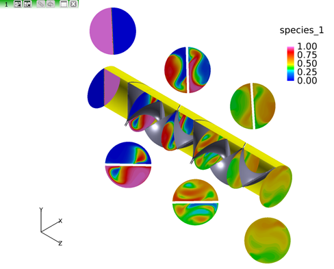
On the Function Selection panel, scroll up (if needed), select species_1 and click Calculate.
Close the Function Specification panel.
On the Colormap tab of the Coordinate Surface panel, adjust the min/max SCALAR COLORING
to 0.00 and 1.00.
Click On the Function Selection panel, scroll down in the list, if needed, select
Conc Variance, and click Calculate to
apply species_1 as the scalar function for all coordinate surfaces.
Figure 20.
Double click the top coordinate surface on the upstream end of the mixer.
Click the
icon.
Click Scalar.
On the Function Selection panel, scroll down in the list (if needed), select
Conc Variance, and click Calculate.
Close the Function Specification panel.
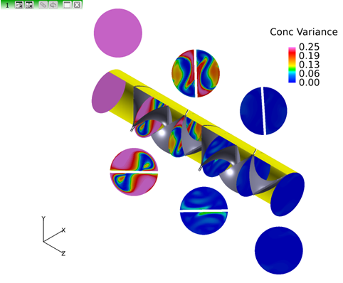
On the Colormap tab of the Coordinate Surface panel, adjust the max/min range to
0.00 and 0.25.
Click Tools > Unify to apply Conc_Variance as the scalar function for all of the coordinate
surfaces.
Figure 21.
Species variance shows the extent of mixing statistically. At the inlet, the fluid is
completely unmixed, and in this case, the variance should be equal to 0.25 (Note:
average concentration throughout the mixer will always be 0.5.) At each of the
cross-sections, the variance decreases. These values can be computed by AcuFieldView.
Section #
Variance (average)
1
0.2312
2
0.1702
3
0.1059
4
0.0193
5
0.0071
6
0.0029
To compute variance for a section, double click a section to make it current.
Click the Integrate icon or Tools > Unify.
Tip: To see the icon on the toolbar, you might need to expand the toolbar with
the
icon.
Change the Integration Mode to Current Surface.
Click Integrate to calculate the integral of the scalar function over the surface.
The following image shows the results for the fifth section (one up from the downstream end of
the mixer). Figure 22.
Create a Keyframe Animation
This section shows how to create a keyframe animation of an exploded view. A keyframe
animation allows for more control of animations and consists of tracks of keyframes and
actions. Tracks exist for each dataset, region and surface. This section uses a complete
restart and a keyframe restart that are provided with the tutorial data. Keyframe
animations require some planning before execution due to the complexity of the animation
that can be created.
Click File > Open Restart > Complete.
In the <your working dir>\polymer_mixing\restart
directory, select KeyStart.dat and click
Open.
This creates an animation file of a standard size that can be converted
to MPEG, if desired.
Click Tools > Keyframe Animation.
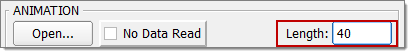
In the ANIMATION section, click Create to create a new keyframe animation.
In the Length field, double click 120, change the
default keyframe animation length to 40, and press
Enter.
The animation will not need to be longer and this will also help display the
time line more clearly. Figure 23.
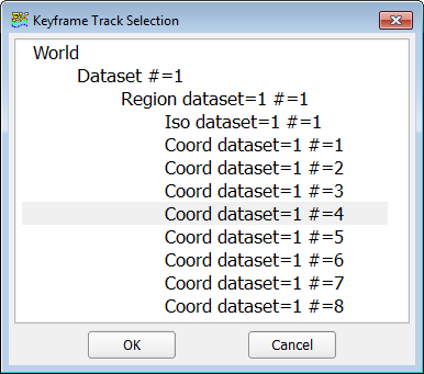
Click Select in the Track section.
In the Keyframe Track Selection panel, select Coord dataset=1 #=4 and click OK.
This selects the coordinate surface with ID = 4 as the surface to be
animated. This is the duplicate surface at the upstream end of the mixer that
was moved up and rotated earlier in this tutorial. Figure 24.
In the FRAME DISPLAY section, move the slider to
40.
In the KEYFRAME section, click Create to create a keyframe at frame 40 for Coord dataset=1 #=4.
Turn on Transformation to set the position of this
particular surface for keyframe number 1, which corresponds to a frame number of
40.
This is the final position of the surface in the animation.
To set the initial position of the surface, set the Current frame to
1 in the FRAME DISPLAY section.
Click Create in the KEYFRAME section.
On the Transform Controls toolbar, click Reset.
This places the surface at its original, untransformed position and
turns on Transformation. This change is not visible until the animation is
played or you click in the modeling window. Figure 25.
Click to preview your animation or the Frame Advance arrows to preview specific
frames.
Tip: To speed up the preview, pause the animation and edit the Inc
value to 2 or to 4 to play only every other or every fourth frame, and play
the animation to see the effect of changing this value.
Pause the animation.
Click Select, select Coord dataset=1
#=6 and click OK to set the two keyframes
for the next coordinate surface.
Change the Current frame to 40 in the FRAME DISPLAY
section.
In the KEYFRAME section, click Create to create a key for the final position of the surface.
Turn on Transformation and change the Current frame to
1.
Click Create in the KEYFRAME section.
On the Transform Controls toolbar, click Reset to set the initial position of the surface.
Repeat the steps above for coordinate surface numbers 8, 10, 12 and 14.
Click Save in the KeyFrame Animation panel.
Name and save the keyframe animation file.
Click File > Save Restart > Complete.
Name and save the complete restart. The complete restart and the keyframe
animation can be loaded into a new AcuFieldView
session so that you can view the animation later.
Click Build Flipbook on the KeyFrame Animation panel to create a keyframe animation file that you can view independently of
AcuFieldView.
Click OK in the Flipbook Size Warning panel.
In the Flipbook Controls panel that opens when the build is complete, click Save.
In the Flipbook File Save browser, name and save the animation file.
This file can be opened independently of AcuFieldView to watch the
animation.
Close the Flipbook Controls panel.
Click File > Open Restart > Complete.
In the <your working dir>\polymer_mixing\restart
directory, select KeyComplete_key.dat and click
Open.
Click Tools > Keyframe Animation to open the KeyFrame Animation panel.
Click Open.
In the <your working dir>\polymer_mixing\restart
directory, select KeyComplete.key and click
Open.
Play the animation.
This keyframe animation contains all of the keyframe transformations that you created earlier
in this tutorial. In addition, an annotation has been added that fades
in.
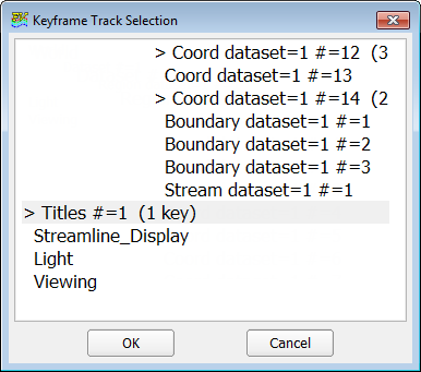
Click Select, scroll down, select Titles #=1 and click OK.
Figure 26.
Click Clear to remove the key for the title.
Play the animation to see the effect of this change.
The title's current position will be its final position.
Pause the animation. Change the Current frame to
8.
Click Create in the KEYFRAME section.
Turn on Transformation and change the Current frame to
1.
Click Create in the KEYFRAME section.
Change the Visibility from On to Fade In.
Note that the fade-in has already started. The fade starts immediately
on frame 1, which has a fade (transparency) value of 0.125.
With Shift + left mouse, move the title closer to the
mixer.
This will automatically turn on the Transformation button and set the
keyframe.
Play the animation.
The annotation should start from the position of the title in the last step and move to the
final position.
Pause the animation.
Change the Frame Number in the KEYFRAME section to
2.
Play the animation.
The title will be invisible at the beginning of the animation, then fade in and move to its
final position.
Click Build Flipbook to create a new keyframe animation file.
In the Flipbook Controls panel that opens when the build is complete, click Save.
Name and save the animation file.
In the KeyFrame Animation panel, click Save.
Name and save the keyframe animation file.
Click File > Save Restart > Complete.
Name and save the complete restart. The complete restart and the keyframe
animation can be loaded into a new AcuFieldView
session so that you can view the animation later.
A complete restart (KeyComplete_key.dat) and a completed
keyframe animation (keyComplete.key) are provided in
<your_working_dir>\ploymer_mixing\restart. This
keyframe animation contains all of the keyframes and actions that are produced
by the above steps.
Click File > Open Restart > Complete.
In the <your working dir>\polymer_mixing\restart
directory, select KeyComplete_key.dat and click
Open.
Click Open on the Keyframe Animation panel.
In the <your working dir>\polymer_mixing\restart
directory, select keyComplete.key and click
Open.
This opens a keyframe animation with a title that fades in and moves
from near the mixer to its current position, but faster than the
surfaces.
Equations for Static Mixer
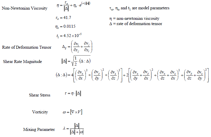
A number of mathematical expressions were used to create the visualizations
presented in this tutorial and have been provided as formula restarts. An
explanation of the equations found in the formula restarts and used in the
tutorial is given here.
The following definitions were used in the static mixer equations: Figure 27.
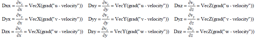
AcuFieldView Equations
In the following equations, the name of the function as stored in the
restart files and as appears in AcuFieldView
when read in is shown first, followed by the mathematical expression
followed by the expression used in AcuFieldView
to define the given function. All of the terms and factors of the
expressions used in AcuFieldView are either
intrinsic functions available on the Function Formula Specification panel or
have been previously defined in this section. Figure 28.
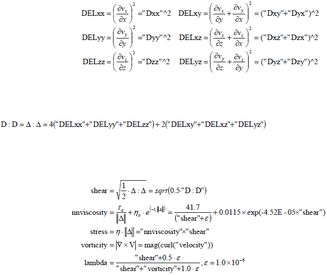
and so on for Dxy, Dyy, Dzy and Dxz, Dyz and Dzz.Figure 29.
 to open the Boundary Surface panel.
 on the toolbar to open the Color Mixer panel.
 to open the Coordinate Surface panel.
 to turn the Outline off.
 and use M1 (left mouse) to select an area to zoom into the third blade
element.
and use M1 (left mouse) to select an area to zoom into the third blade
element.
 to open the Iso-Surface panel.
 or to open the Streamlines panel.
 to activate the locked transformation controls.

 , you can click the toolbar icons to transform
the surface. When the mouse icon has a darker background
, you can click the toolbar icons to transform
the surface. When the mouse icon has a darker background  , you can perform transformation by clicking a pair of toolbar
icons and then using the right mouse to transform the surface.
, you can perform transformation by clicking a pair of toolbar
icons and then using the right mouse to transform the surface.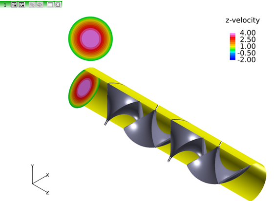
 on the Viewer toolbar to toggle to Locked
Transforms control and move the coordinate surface up.
on the Viewer toolbar to toggle to Locked
Transforms control and move the coordinate surface up.
 icon.
icon.
 or .
Tip: To see the icon on the toolbar, you might need to expand the toolbar with the
or .
Tip: To see the icon on the toolbar, you might need to expand the toolbar with the icon.
icon.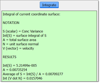

 to preview your animation or the Frame Advance arrows to preview specific
frames.
Tip: To speed up the preview, pause the animation and edit the Inc value to 2 or to 4 to play only every other or every fourth frame, and play the animation to see the effect of changing this value.
to preview your animation or the Frame Advance arrows to preview specific
frames.
Tip: To speed up the preview, pause the animation and edit the Inc value to 2 or to 4 to play only every other or every fourth frame, and play the animation to see the effect of changing this value.