This tutorial looks at an application from the biomedical industry. A catheter is
inserted into an artery with a tumor. The injection of a drug through the catheter into the
artery and its absorption into the tumor is investigated.
Prior to running this tutorial, copy the expanded biomedical
directory from <AcuSolve installation
directory>\model_files\tutorials\AcuFieldView\AFV_tutorial_inputs.zip
to a working directory. See Tutorial Data for more information.
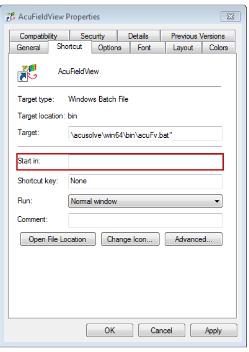
For Windows users, in order to take advantage of the restarts provided for this
tutorial, you will need to make sure that the properties for your AcuFieldView shortcut on the Start menu do not include a
Start in entry. To change that property, browse to the AcuFieldView shortcut on the Start menu, right-click, and
select Properties. The Start in field can be found on the
Shortcut tab in the AcuFieldView Properties dialog. Note
that this step is only necessary because the restart files use relative paths. Figure 1.
Solve the Case with AcuConsole and AcuSolve
Start
AcuConsole.
Open <your working
dir>\biomedical\biomedical.acs.
Run
AcuSolve to calculate a solution.
Exit
AcuConsole.
Start AcuFieldView and Load the Data
Start
AcuFieldView.
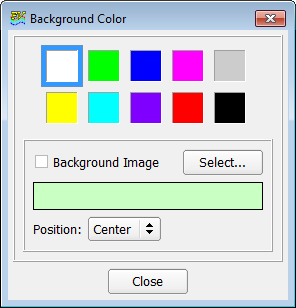
Click View > Background Color and select white.
Figure 2.
Click Close.
Click File > Data Input > AcuSolve [Direct Reader].
Click Read Grids & Results Data.
Browse to the \biomedical directory, select
biomedical.1.log, and click
Open.
In the Function Subset Selection panel, which opens with all functions selected
by default, click OK.
When the data has loaded, switch the INPUT MODE to
Append.
Read biomedical.1.Log again and close the AcuSolve [Direct Reader] panel once the data has loaded a
second time.
On the main toolbar, click Dataset.
Set SCALE X to -1.
Click Apply and Close.
Dataset 2 now mirrors dataset 1 along the X plane.
On the main toolbar change the value for Dataset to 1 to
set the dataset that you loaded first as the current dataset.
Tip: You can also change the current dataset on the Dataset Controls
panel.
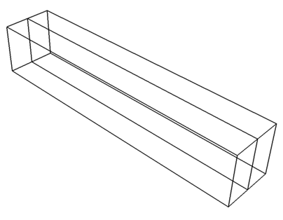
Click Bound to
open the Boundary Surface panel.
Click Create, select OSF: Tumor
Walls in the BOUNDARY TYPE list and click
OK.
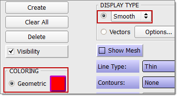
Change DISPLAY TYPE to Smooth shading and Geometric
COLORING to red.
Figure 3.
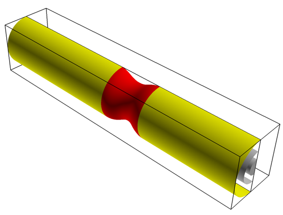
Create a second surface consisting of OSF: Artery Walls with Geometric COLORING
yellow.
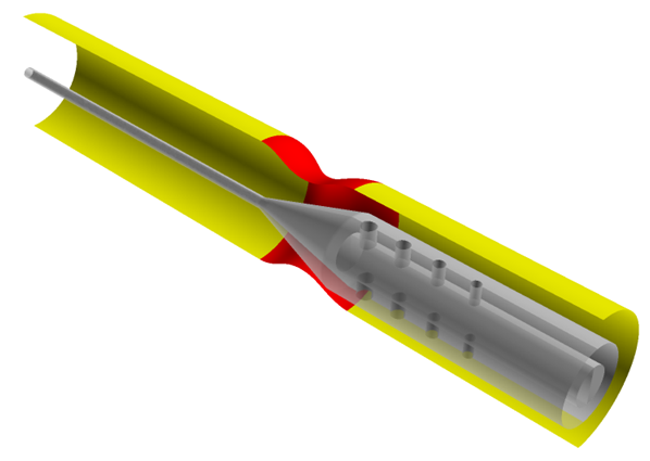
Create a third surface consisting of OSF: Catheter Inlet and OSF: Catheter
Walls with Geometric COLORING gray.
Figure 4.
Click File > Save Restart > Current Dataset.
Browse to the \biomedical\restart directory, name the file
tumor_1, and click Save.
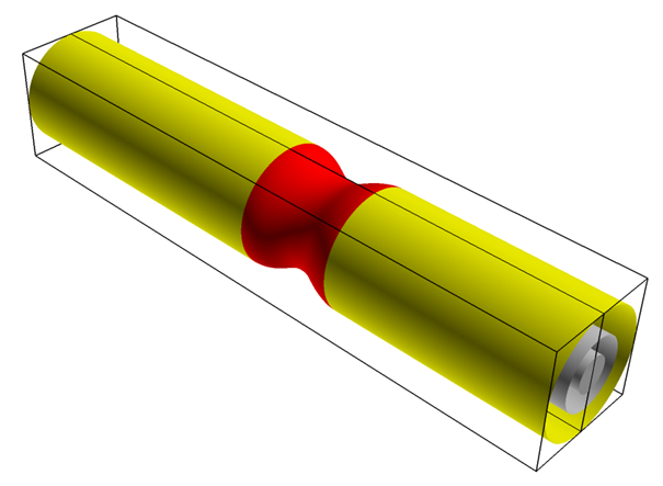
Make Dataset 2 current using the control on the toolbar or by clicking
Dataset and changing the ID on the Dataset Controls
panel.
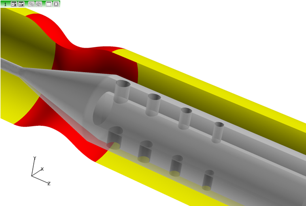
Click File > Open Restart > Current Dataset and open tumor_1.dat to create the same
three surfaces on dataset 2 as on dataset 1.
Figure 5.
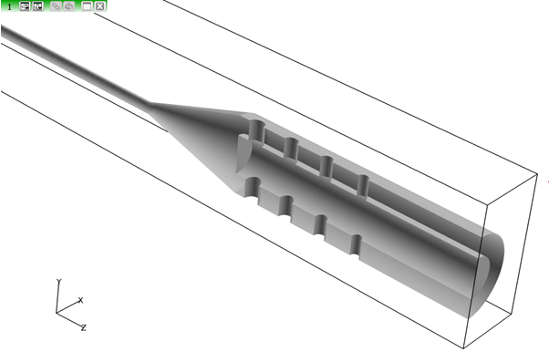
Change the current Dataset to 1.
On the Boundary Surface panel, set the Surface ID to
1.
Turn off the Visibility of the tumor walls.
Set the Surface ID to 2 and turn off the Visibility of
the artery walls.
Set the Surface ID to 3 off and set the Transparency to
50.0%.
This will make the catheter inlet and walls partially
transparent.
On the Transform Controls toolbar, turn the Outline display off by clicking the
icon.
Figure 6.
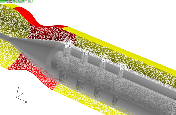
Visualize the Flow Field
In this step you will create a vector coordinate surface to visualize the flow field created by the interaction of the fluid carrying the drug with the blood in the artery.
Rotate the view slightly and zoom into the catheter ports and the tumor.
Figure 7.
Click File > Open Restart > Formula.
In the ..\biomedical\restart directory, select
bio.frm and click Open.
Click Dataset on the toolbar to open the Dataset
Controls panel.
Make sure that the Dataset is set to 2.
Click Coord
to open the Coordinate Surface panel.
Click Create and set the COORD PLANE to
X.
Enter -1e-005 for the Current position in the COORD
PLANE section.
Change the DISPLAY TYPE to Vectors.
For Vector Function, click Select.
In the Function Selection panel, select
nrmlz('velocity') and click
Calculate.
Click Options in the Coordinate Surface panel to open
the Vector Options panel.
Turn on Head Scaling and change the value to
0.125.
Change the TYPE from Total to Projected.
Activate the Skip option and change it to
87.5 %.
Change the Length Scale to 0.25.
Close the Vector Options panel.
Change the Geometric COLORING to white.
Figure 8.
Set the current Dataset to 1. Turn off Visibility for
dataset 1.
Only the boundary and coordinate surfaces for dataset 2 will be
visible. Figure 9.
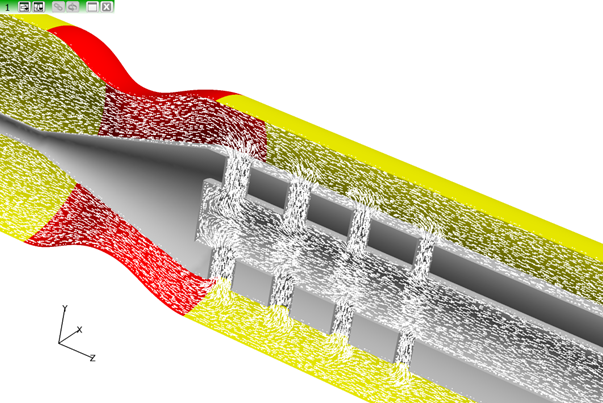
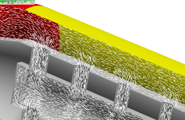
Click Zoom.
Use the left mouse button (M1) to drag a rectangular zoom box around a few of
the catheter ports. The vectors indicate the flow direction and velocity of
blood flow in the artery as well as the flow of drug-containing fluid in the
catheter. Notice the change in direction as the fluid moves through the catheter
into the delivery ports. Also notice the flow interaction between the fluid
containing the drug and the blood flow through the artery.
Figure 10.
Click Undo Zoom
to reset the view.
Tip: You can undo the zoom again to reset the view to an earlier
zoom. Use the right mouse button to change the zoom by dragging in the
visualization window.
Display the Shear on the Artery Wall
In this step you will see the shear on the artery wall created by the drug release through
the holes of the catheter.
Double click the Artery
Wall to set the dataset to
2 and open the Boundary
Surface panel with the Surface ID set to 2.
For Scalar Function, click
Select.
In the Function Selection panel, scroll down
and select shear.
Click Calculate.
Change COLORING from Geometric to
Scalar.
In the Colormap tab, change the minimum to
100, the maximum to
500 and the Number of
Contours to 32.
Turn on Filled Contour.
Click Tools > Unify to make all the surfaces of the
same type (boundary) and of the current dataset
(dataset 2) display shear with the set color
ranges.
Notice the very high shear rates on the artery
wall due to the delivery of the drug through the
holes of the catheter. This shows an undesirable
amount of shear on the artery.
Figure 11.
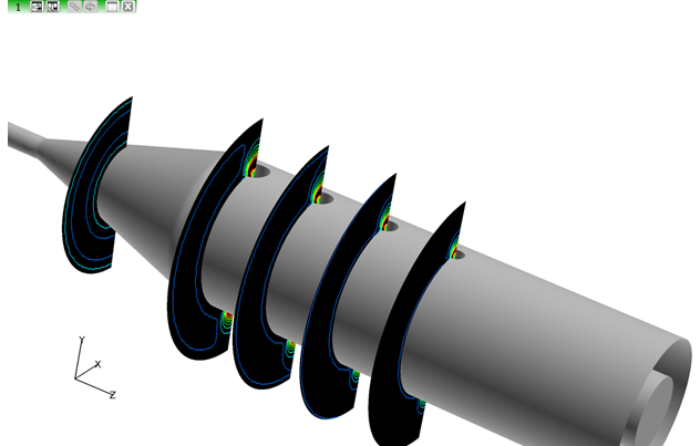
Visualize Stress and Concentration Contours
In this step you will see stress contours and concentration contours at and near the
location of the catheter ports. For each set of planes, you will see a different way to
create multiple surfaces of the same type.
Double-click the vectors to open the Coordinate Surface panel.
Turn Visibility off.
Double-click the artery surface to open the Boundary Surface panel.
Turn Visibility off for the artery walls.
Change the Surface ID to 1
and turn Visibility off for the tumor walls.
Double-click on the catheter boundary surface and change to Geometric COLORING.
Figure 12.
Change the Dataset to make dataset 1 current, and turn the Visibility on.
Double-click the Catheter boundary surface for dataset 1 and set the Transparency back
to 0.
While dataset 1 is current, click to open the
Coordinate Surface panel.
Create a coordinate surface.
Turn Visibility on. Set the COORD PLANE to
Z and the Current position to
-0.0001.
Create four more coordinate surfaces: at Z= -0.0003,
-0.0005, -0.0007 and
-0.0011.
Change the DISPLAY TYPE of the current surface (Z=-0.0011) to
Constant shading.
Change the Geometric COLORING to black, Contours from None to
Scalar and Scalar Function to
stress.
On the Colormap tab, change the minimum to 0.0, the maximum to 180.0 and the Number of Contours to 10.
Click Tools > Unify to make all the surfaces of the same type (coordinate) and of the current
dataset (dataset 1) display stress with the set color ranges.
Figure 13.
Click File > Save Restart > Current Dataset and save a Current Dataset restart named
tumor_2.dat.
Make dataset 2 current by changing the Dataset value on the toolbar.
Click File > Open Restart > Current Dataset and open the Current Dataset restart to create the same five surfaces on
dataset 2 as on dataset 1.
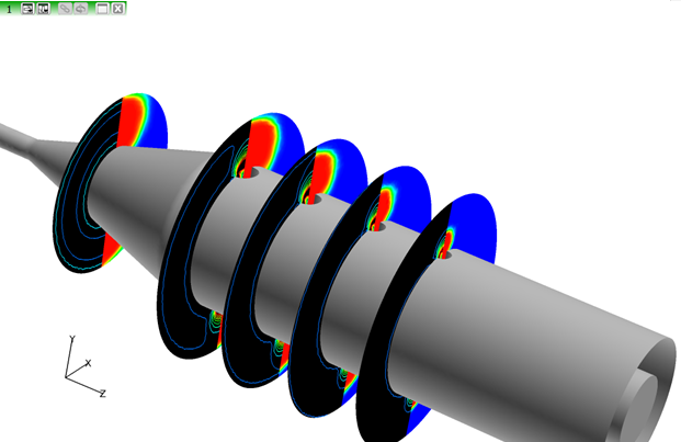
Double-click one coordinate surface in dataset 2.
Change the Scalar Function to species_1 and COLORING to
Scalar.
Click Tools > Unify to propagate the change to the other four surfaces.
Figure 14.
Calculate the Mass Balance
In this step you will calculate the mass balance of the solution by taking into
consideration both the convective flux through the artery as well as the diffusive flux
through the artery wall and the tumor.
Double-click a scalar surface to open the Coordinate Surface panel.
Click Clear All and then click OK.
This will clear all coordinate surfaces on one of the datasets.
Double click any of the remaining species_1 surfaces to open the Coordinate Surface panel.
Click Clear All and then click OK on the
Coordinate Surface: Clear All Confirmation panel.
This will clear all coordinate surfaces on the other dataset.
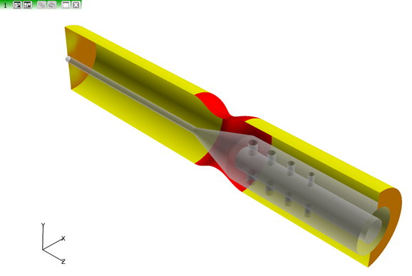
For boundary surface 3 of both datasets, turn on the Visibility and change the
Transparency to 50.0%.
For dataset 2, turn on the Visibility of boundary surfaces 1 and 2.
For dataset 2, create a fourth boundary surface.
Select Blood Inlet and click OK.
Change COLORING to Scalar.
Change the Scalar Function to Nconvective to show the convective flux into the artery.
Create a fifth boundary surface using Blood Outlet.
This surface has the Scalar Function already set to Nconvective.
Zoom out to show the whole model.
Rotate the view so that you can see the upstream end of the model.
Figure 15.
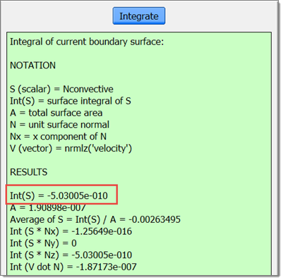
Click Tools > Integration to open the Integration Controls panel.
Change the Integration Mode to Current Surface.
Click Integrate.
The convective flux out of the artery Int(S) is about -5.03 e-010. Integrating across this
surface gives an indication of the relative amount of drug that flows out of the artery.
Figure 16.
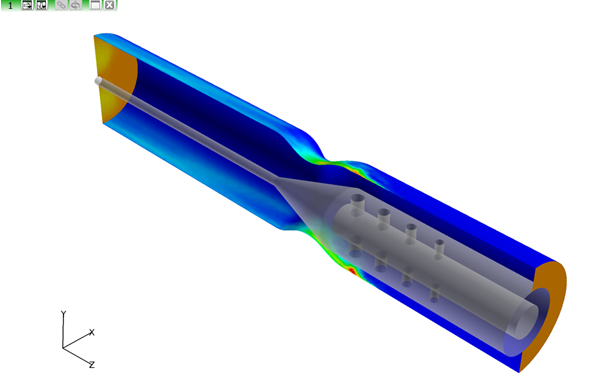
For boundary surface 2 (Artery Walls), change the COLORING to Scalar and change the Scalar Function to Ndiff-Normal, the diffusive flux into the wall.
On the Colormap tab, change the min and max to 0.0 and
2000.0.
Integrate to get around 2.33e-004.
Integrating on this surface indicates the relative amount of the drug that is
impinging on the artery walls.
Switch to boundary surface 1 (Tumor Walls).
Change the COLORING to Scalar and change the Scalar Function to
Ndiff-Normal. On the Colormap tab, change the min and max to
0.0 and 2000.0.
Turn on Visibility.
Integrate to get about 9.77e-005.
Integrating on this surface indicates the relative amount of the drug that is
impinging on the tumor wall. Comparison of the integrated values for the artery walls and
the tumor walls indicates that for this model greater than twice the amount of the drug
diffuses into the artery walls compared to the drug that diffuses into the tumor wall. Figure 17.
Visualize the Drug Delivery
In this step you will look at the flow of the medicine and show some visualization
"tricks".
For dataset 1, boundary surface 3 (Catheter Inlet and Catheter Walls), set the Transparency to 0.
Double-click the Artery Wall (dataset 2, boundary surface 2) and change the COLORING to
Geometric (yellow).
Click Tools > Color Mixer or on the toolbar.
Click the yellow chip. Change the Red, Green
and Blue values to 235,
182, and
180.
Click Apply and
Close.
Change to Dataset 1 and click Iso to open
the Iso-Surface panel.
Click Create.
Click Select next to Iso
Function.
Select species_1 on the
Function Selection panel and click
Calculate.
Set the Current value for Iso Function to 0.5 and make the color blue.
Change the DISPLAY TYPE to
Smooth shading.
Open the Color Mixer and change the blue color
chip RGB values to 212,
212,
0.
Click Apply and
Close.
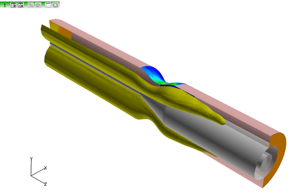
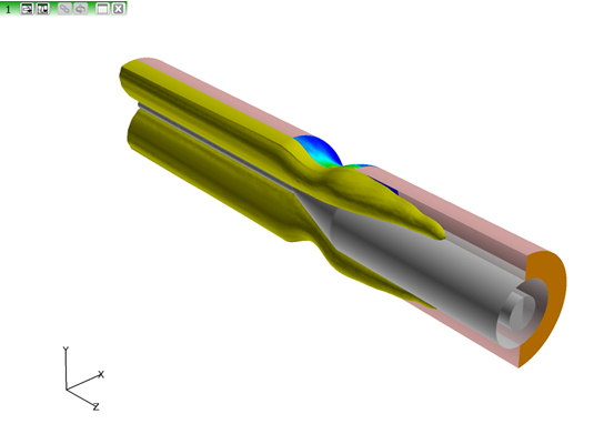
Figure 18.
The iso-surface intersecting the artery wall is
open. To close it, create a fourth boundary
surface on dataset 1 consisting of OSF: Artery
Walls, OSF: Tumor Walls. Color it dark
yellow.
For Threshold Function, click
Select.
On the Function Selection panel, select
species _1 and click
Calculate.
Turn Threshold Clip on and set Min to 0.5 to fill in the "open top" and clip the rest.
 to
open the Boundary Surface panel.
to
open the Boundary Surface panel.
 icon.
icon.
 to open the Coordinate Surface panel.
 .
.
 to reset the view.
Tip: You can undo the zoom again to reset the view to an earlier zoom. Use the right mouse button to change the zoom by dragging in the visualization window.
to reset the view.
Tip: You can undo the zoom again to reset the view to an earlier zoom. Use the right mouse button to change the zoom by dragging in the visualization window.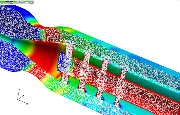
 on the toolbar.
 to open
the Iso-Surface panel.
to open
the Iso-Surface panel.