Turbulent Flow Over a NACA 0012 Airfoil
In this application, AcuSolve is used to simulate turbulent flow of a fluid over a NACA 0012 airfoil at 3 angles of attack, 0 degrees, 10 degrees, and 15 degrees. AcuSolve results are compared with experimental results for coefficients of pressure, lift, and drag reported by NASA. The close agreement of AcuSolve results with experimental results validates the ability of AcuSolve to model external aerodynamics.
Problem Description
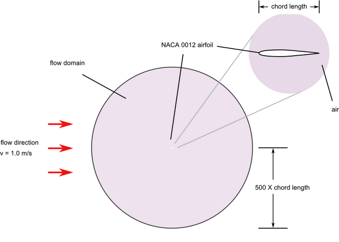
Figure 1. Critical Dimensions and Parameters for Simulating Turbulent Flow over a NACA 0012 Airfoil
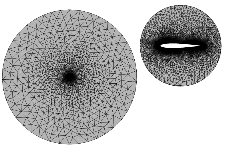
Figure 2. Mesh Used for Simulating Turbulent Flow over a NACA 0012 Airfoil (the Image on the Left Represents the Full Mesh, the Image on the Right Represents Mesh Details near the Airfoil)
AcuSolve Results
The AcuSolve solution converged to a steady state and the results reflect the mean flow conditions for each of the three angles of attack, 0 degrees, 10 degrees, and 15 degrees. For each case, the angle of attack was varied by changing the angle of the incident flow. Note that this enables the use of a single mesh for all of the simulations.
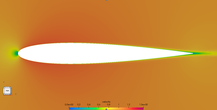
Figure 3. Contours of Velocity Magnitude Where Angle of Attack = 0 Degrees
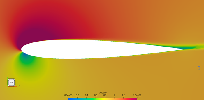
Figure 4. Contours of Velocity Magnitude Where Angle of Attack = 10 degrees
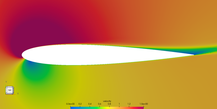
Figure 5. Contours of Velocity Magnitude Where Angle of Attack = 15 Degrees
| CL (α=10) | CL (α=15) | cd (α=0) | cd (α=10) | cd (α=15) | |
|---|---|---|---|---|---|
| Experimental | 1.0941 | 1.5576 | 0.0082 | 0.0123 | 0.0207 |
| AcuSolve | 1.0905 | 1.5428 | 0.0081 | 0.0124 | 0.0208 |
| Percent deviation from experimental | 0.33 | 0.95 | 1.22 | 0.81 | 0.48 |
AcuSolve values for coefficient of pressure are plotted against experimental results for angles of attack (α) of 0 degrees, 10 degrees, and 15 degrees in the following plots. The results are presented for normalized distance along the airfoil, given by x/c, where x is the distance from the leading edge and c is the chord length.
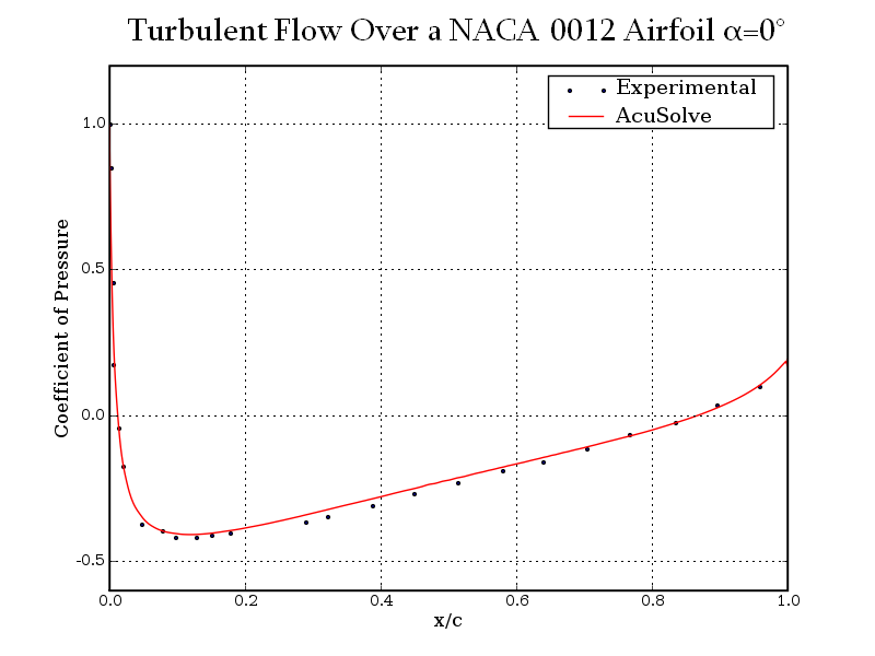
Figure 6. Coefficient of Pressure Plotted Against Normalized Distance Along the Airfoil for Angle of Attack (α) = 0 Degrees
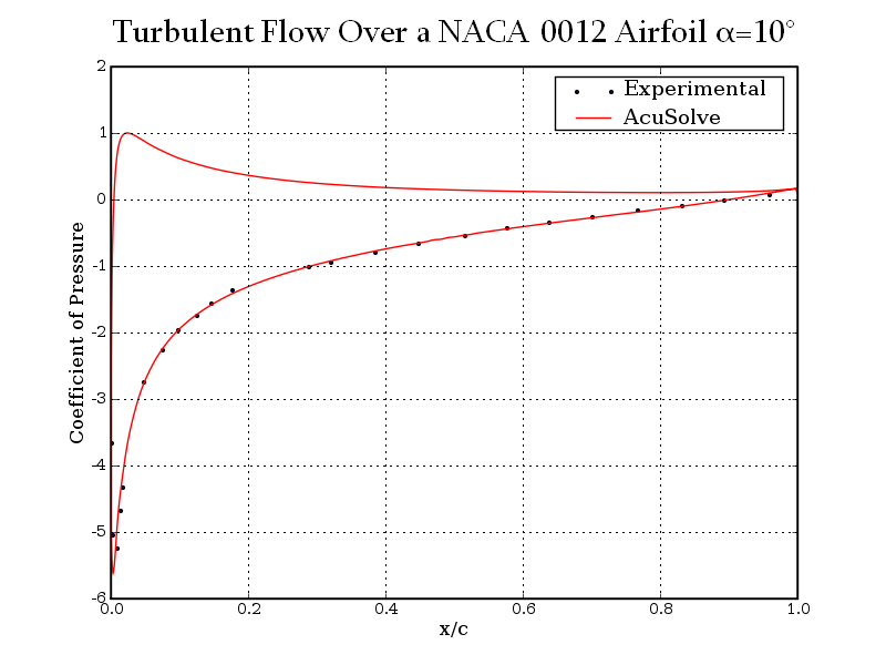
Figure 7. Coefficient of Pressure Plotted Against Normalized Distance Along the Airfoil For Angle of Attack (α) = 10 Degrees
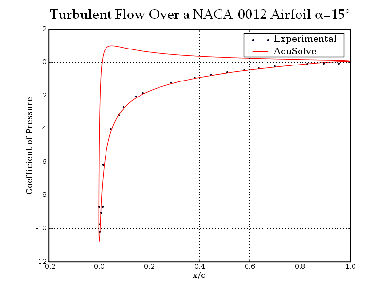
Figure 8. Coefficient of Pressure Plotted Against Normalized Distance Along the Airfoil for Angle of Attack (α) = 15 Degrees
Summary
The AcuSolve results compare well with the experimental results for flow over a NACA 0012 airfoil. In this application, a constant-velocity flow field impinges on the airfoil surface. As the flow convects in the streamwise direction along the airfoil surface, a boundary layer develops. The rate at which the boundary layer develops has significant impact on the viscous stresses present on the airfoil surface. At low angles of attack these stresses dominate the drag on the airfoil. As the angle of attack increases, the flow over the airfoil is no longer symmetric, which leads to the generation of lift. For non-zero angles of attack, the asymmetric pressure distribution on the airfoil creates another source of drag that is combined with the viscous stresses to determine the total drag on the airfoil. The AcuSolve results for coefficients of lift and drag at the 15 percent angle of attack are within 0.91 percent and 0.5 percent of experimental values, respectively. AcuSolve results for coefficient of pressure closely agree with experimental results along the length of the airfoil for all three angles of attack that were investigated.
Simulation Settings for Turbulent Flow Over a NACA0012 Airfoil
HyperWorks CFD database file: <your working directory>\airfoil_turbulent\airfoil_turbulent.hm
Global
- Problem Description
- Analysis type - Steady State
- Turbulence equation - Spalart Allmaras
- Auto Solution Strategy
- Convergence tolerance - 0.0001
- Relaxation factor - 0.4
- Material Model
- Fluid
- Density - 1.0 kg/m3
- Viscosity - 1.667e-7 kg/m-sec
Model
- Fluid
- Volumes
- Fluid
- Element Set
- Material model - Fluid
- Element Set
- Fluid
- Surfaces
- +z slip
- Simple Boundary Condition
- Type - Slip
- Simple Boundary Condition
- -z slip
- Simple Boundary Condition
- Type - Slip
- Simple Boundary Condition
- airfoil surface
- Simple Boundary Condition
- Type - Wall
- Simple Boundary Condition
- farfield
- Simple Boundary Condition
- Type - Far Field
- X velocity - cos(α) m/sec
- Y velocity - sin(α) m/sec
- Simple Boundary Condition
- +z slip
- Eddy viscosity - 1.0e-9 m2/sec
References
NASA - Langley Research Center. http://turbmodels.larc.nasa.gov/naca0012_val_sa.html