DENSITY_MODEL
Specifies a density model.
Type
AcuSolve Command
Syntax
DENSITY_MODEL("name") {parameters...}
Qualifier
User-given name.
Parameters
- type (enumerated) [=none]
- Type of the density model.
- constant or const
- Constant density. Requires density.
- boussinesq
- Boussinesq approximation. Requires density, expansivity_type and reference_temperature.
- isentropic
- Isentropic gas. Requires density, specific_heat_ratio and reference_pressure, and also absolute_pressure_offset from the EQUATION command.
- ideal_gas
- Ideal gas law. Requires gas_constant, and also absolute_pressure_offset and absolute_temperature_offset from the EQUATION command.
- piecewise_linear or linear
- Piecewise linear curve fit. Requires curve_fit_values and curve_fit_variable.
- cubic_spline or spline
- Cubic spline curve fit. Requires curve_fit_values and curve_fit_variable.
- user_function or user
- User-defined function. Requires user_function, user_values and user_strings.
- density or dens (real) >0 [=1]
- Constant value of the density when used with constant and boussinesq types, and value of the reference density when used with isentropic type.
- expansivity_type or expans_type (enumerated) [=constant]
- Type of the expansivity function used for the Boussinesq approximation. Used with
boussinesq type.
- constant or const
- Constant expansivity. Requires expansivity.
- expansivity or expans (real) >=0 [=1]
- Constant value of the expansivity. Used with constant expansivity type.
- reference_temperature or ref_temp (real) [=273.15]
- Reference temperature of the Boussinesq approximation. Used with boussinesq type.
- reference_pressure or ref_pres (real) [=0]
- Value of the reference pressure. Used with isentropic type.
- specific_heat_ratio (real) >=1 [=1.4]
- Value of the specific heat ratio. Used with isentropic type.
- gas_constant (real) [=287.058]
- Value of the gas constant. Used with ideal_gas type.
- isothermal_compressibility (real) >=0 [=0]
- Value of the isothermal compressibility.
- curve_fit_values or curve_values (array) [={0,0}]
- A two-column array of independent-variable/density data values. Used with piecewise_linear and cubic_spline types.
- curve_fit_variable or curve_var (enumerated) [=temperature]
- Independent variable of the curve fit. Used with piecewise_linear and
cubic_spline types.
- x_coordinate or xcrd
- X-component of coordinates.
- y_coordinate or ycrd
- Y-component of coordinates.
- z_coordinate or zcrd
- Z-component of coordinates.
- x_reference_coordinate or xrefcrd
- X-component of reference coordinates.
- y_reference_coordinate or yrefcrd
- Y-component of reference coordinates.
- z_reference_coordinate or zrefcrd
- Z-component of reference coordinates.
- pressure or pres
- Pressure.
- temperature or temp
- Temperature.
- species_1 or spec1
- Species 1.
- species_2 or spec2
- Species 2.
- species_3 or spec3
- Species 3.
- species_4 or spec4
- Species 4.
- species_5 or spec5
- Species 5.
- species_6 or spec6
- Species 6.
- species_7 or spec7
- Species 7.
- species_8 or spec8
- Species 8.
- species_9 or spec9
- Species 9.
- user_function or user (string) [no default]
- Name of the user-defined function. Used with user_function type.
- user_values (array) [={}]
- Array of values to be passed to the user-defined function. Used with user_function type.
- user_strings (list) [={}]
- Array of strings to be passed to the user-defined function. Used with user_function type.
Description
This command specifies a density model for element sets. All types of element sets, fluid, solid, and shell, require a density model.
DENSITY_MODEL( "my density model" ) {
   type                                = constant
   density                             = 1.225
   isothermal_compressibility          = 0
 }
 MATERIAL_MODEL( "my material model" ) {
   density_model                       = "my density model"
   ...
 }
 ELEMENT_SET( "fluid elements" ) {
   material_model                      = "my material model"
   ...
}
A constant density model uses a constant density for the entire element set, as in the above example.
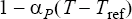
 is the thermal
expansivity, given by expansivity; T
is the temperature; and
is the thermal
expansivity, given by expansivity; T
is the temperature; and  is the temperature at
which the density equals the given constant density value, given by
reference_temperature. For
example,
is the temperature at
which the density equals the given constant density value, given by
reference_temperature. For
example,DENSITY_MODEL( "air" ) {
type = boussinesq
density = 1.225
expansivity_type = constant
expansivity = 0.0034722
reference_temperature = 288
}The Boussinesq model assumes that the problem contains a temperature field; see the EQUATION command. If the problem does not contain any temperature equation, then a boussinesq density model is internally converted to a constant density model.
DENSITY_MODEL( "isentropic air" ) {
   type                    = isentropic
   density                 = 1.225
   specific_heat_ratio     = 1.4
   reference_pressure      = 0
}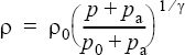
where is the density, given by this command; o is the reference density, given by density; p is the pressure; po is the reference pressure, given by reference_pressure; is the specific heat ratio, given by specific_heat_ratio; and pa is the absolute pressure offset, given by absolute_pressure_offset from the EQUATION command.
where is the specific heat capacity; T is the temperature; R is the gas constant.
DENSITY_MODEL( "ideal gas air" ) {
   type              = ideal_gas
   gas_constant      = 287.058
}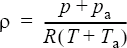
where
is the density, given by this command;
R is the gas constant, given by
gas_constant; p is the pressure;
T is the temperature; and  and
and  are the absolute
pressure and temperature offsets, given by absolute_pressure_offset and
absolute_temperature_offset from the EQUATION
command. This model requires the availability of the temperature field; an error will be
issued otherwise.
are the absolute
pressure and temperature offsets, given by absolute_pressure_offset and
absolute_temperature_offset from the EQUATION
command. This model requires the availability of the temperature field; an error will be
issued otherwise.
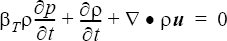
 is the
isothermal compressibility, given by isothermal_compressibility;
is density; p is pressure;
t is time; and
u is the velocity vector. Isothermal
compressibility is defined by:
is the
isothermal compressibility, given by isothermal_compressibility;
is density; p is pressure;
t is time; and
u is the velocity vector. Isothermal
compressibility is defined by:
Pseudo compressibility is often used along with constant type to model wind-generated noise. Pseudo compressibility should not be activated for flow = compressible_navier_stokes.
Full variable-density models are also supported by the piecewise_linear, cubic_spline, and user_function types. As opposed to the Boussinesq type, the density for these types is variable in all terms.
DENSITY_MODEL( "air" ) {
   type                      = piecewise_linear
   curve_fit_values          = { 60, 1.05943 ;
                                160, 0.814836 ;
                                260, 0.662024 ;
                                360, 0.557587 ; }
   curve_fit_variable      = temperature
}
gives a density model by defining density as a function of temperature. Use caution when defining density as a function of pressure; this can easily lead to instability.
The curve_fit_values is a two-column array corresponding to the independent variable, temperature, in this case, and density. The independent variable values must be in ascending order. The limit point values of the curve fit are used when curve_fit_variable falls outside of the curve fit limits.
60      1.05943
160     0.814836
260     0.662024
360 0.557587DENSITY_MODEL( "air" ) {
type = piecewise_linear
curve_fit_values = Read ( "density.mks" )
curve_fit_variable = temperature
}A density of type user_function may be used to model more complex behaviors; see the AcuSolve User-Defined Functions Manual for a detailed description of user-defined functions.
DENSITY_MODEL( "thermal air" ) {
   type                 = user_function
   user_function        = "usrDensity"
   user_values          = { 1.225,         # reference density
                              288,         # reference temperature
                            0.0034722 }    # expansivity
}#include "acusim.h"
#include "udf.h"
UDF_PROTOTYPE( usrDensity ) ; /* function prototype */
Void usrDensity (
UdfHd udfHd, /* Opaque handle for accessing data */
Real* outVec, /* Output vector */
Integer nItems, /* Number of elements */
Integer vecDim /* = 1 */
) {
Real expn ; /* expansivity */
Real rho0 ; /* reference density */
Real rhoMin ; /* minimum density */
Real rhoMax ; /* maximum density */
Real temp0 ; /* reference temperature */
Integer i ; /* a running index */
Real* densJacTemp ; /* partial dens / partial temp */
Real* temp ; /* temperature */
Real* usrVals ; /* user supplied values */
udfCheckNumUsrVals( udfHd, 3 ) ; /* check for error */
usrVals = udfGetUsrVals( udfHd ) ;
rho0 = usrVals[0] ;
temp0 = usrVals[1] ;
expn = usrVals[2] ;
rhoMin = rho0 * (1 - 10 * expn ) ;
rhoMax = rho0 * (1 + 10 * expn ) ;
temp = udfGetElmData( udfHd, UDF_ELM_TEMPERATURE ) ;
densJacTemp = udfGetElmJac( udfHd, UDF_ELM_JAC_TEMPERATURE )
for ( i = 0 ; i < nItems ; i++ ) {
densJacTemp[i] = -rho0 * expn ;
outVec[i] = rho0 * ( 1 + expn * (temp0 - temp[i]) ) ;
if ( outVec[i] < rhoMin ) {
densJacTemp[i] = 0 ;
outVec[i] = rhoMin ;
if ( outVec[i] > rhoMax ) {
densJacTemp[i] = 0 ;
outVec[i] = rhoMax ;
}
} /* end of usrDensity() */The dimensions of the returned density vector, outVec, and the Jacobian vector, densJacTemp, are the number of elements.