Lagrangian and Corotational Formulations

Finite element discretizations with Lagrangian meshes are commonly classified as either an updated Lagrangian formulation or a total Lagrangian formulation. Both formulations use a Lagrangian description. That means that the dependent variables are functions of the material (Lagrangian) coordinates and time. In the geometrically nonlinear structural analysis the configuration of the structure must be tracked in time. This tracking process necessary involves a kinematic description with respect to a reference state. Three choices called "kinematic descriptions" have been extensively used:
Total Lagrangian description (TL)
The FEM equations are formulated with respect to a fixed reference configuration which is not changed throughout the analysis. The initial configuration is often used; but in special cases the reference could be an artificial base configuration.
Updated Lagrangian description (UL)
The reference is the last known (accepted) solution. It is kept fixed over a step and updated at the end of each step.
Corotational description (CR)
The FEM equations of each element are referred to two systems. A fixed or base configuration is used as in TL to compute the rigid body motion of the element. Then the deformed current state is referred to the corotated configuration obtained by the rigid body motion of the initial reference.
The updated Lagrangian and corotational formulations are the approaches used in Radioss. These two approaches are schematically presented in Figure 1.


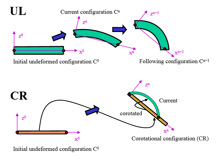
Figure 1. Updated Lagrangian and Corotational Descriptions

By default, Radioss uses a large strain, large displacement formulation with explicit time integration. The large displacement formulation is obtained by computing the derivative of the shape functions at each cycle. The large strain formulation is derived from the incremental strain computation. Hence, stress and strains are true stresses and true strains.

In the updated Lagrangian formulation, the Lagrangian coordinates are considered instantaneously coincident with the Eulerian spatial x MathType@MTEF@5@5@+= feaagKart1ev2aaatCvAUfeBSjuyZL2yd9gzLbvyNv2CaerbuLwBLn hiov2DGi1BTfMBaeXatLxBI9gBaerbd9wDYLwzYbItLDharqqtubsr 4rNCHbGeaGqiVu0Je9sqqrpepC0xbbL8F4rqqrFfpeea0xe9Lq=Jc9 vqaqpepm0xbba9pwe9Q8fs0=yqaqpepae9pg0FirpepeKkFr0xfr=x fr=xb9adbaqaaeGaciGaaiaabeqaamaabaabaaGcbiqaaWgdcaWG4b aaaa@376E@ coordinates. This leads to the following simplifications:(1)
x i X j = X j x i = δ i j
(2)
d Ω = d Ω 0

The derivatives are with respect to the spatial (Eulerian) coordinates. The weak form involves integrals over the deformed or current configuration. In the total Lagrangian formulation, the weak form involves integrals over the initial (reference) configuration and derivatives are taken with respect to the material coordinates.

The corotational kinematic description is the most recent of the formulations in geometrically nonlinear structural analysis. It decouples small strain material nonlinearities from geometric nonlinearities and handles naturally the question of frame indifference of anisotropic behavior due to fabrication or material nonlinearities. Several important works outline the various versions of CR formulation. 1 2 3 4 5

Some new generation of Radioss elements are based on this approach. Refer to Element Library for more details.
Note: A similar approach to CR description using convected-coordinates is used in some branches of fluid mechanics and theology. However, the CR description maintains orthogonality of the moving frames. This will allow achieving an exact decomposition of rigid body motion and deformational modes. On the other hand, convected coordinates form a curvilinear system that fits the change of metric as the body deforms. The difference tends to disappear as the mesh becomes finer. However, in general case the CR approach is more convenient in structural mechanics.

1 Belytschko T. and Hsieh B.H., “Nonlinear Transient Finite Element Analysis with convected coordinates”, Int. Journal Num. Methods in Engineering, 7 255-271, 1973.
2 Argyris J.H., “An excursion into the large rotations”, Computer Methods in Applied Mechanics and Engineering, 32, 85-155, 1982.
3 Crisfield M.A., “A consistent corotational formulation for nonlinear three-dimensional beam element”, Computer Methods in Applied Mechanics and Engineering, 81, 131-150, 1990.
4 Simo J.C., “A finite strain beam formulation, Part I: The three-dimensional dynamic problem”, Computer Methods in Applied Mechanics and Engineering, 49, 55-70, 1985.
5 Wempner G.A., “F.E., finite rotations and small strains of flexible shells”, IJSS, 5, 117-153, 1969.