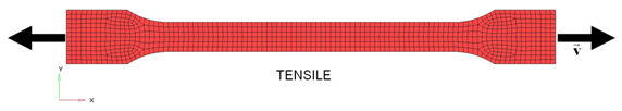
This tutorial demonstrates how to simulate a uniaxial tensile test using a quarter
size mesh with symmetric boundary conditions.
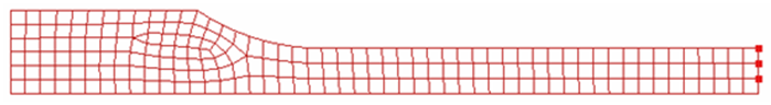
Figure 1.
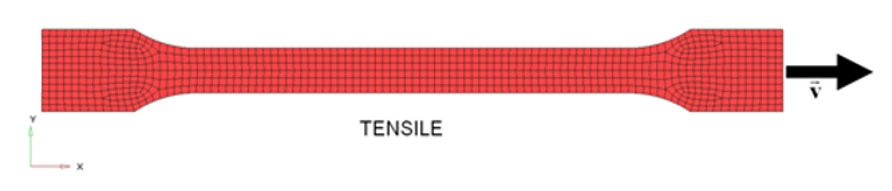
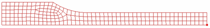
The model is reduced to one-quarter of the total mesh with symmetric boundary
conditions to simulate the presence of the rest of the part. Figure 2.
The model description is as follows:
UNITS: Length (mm), Time (ms), Mass (kg), Force (kN) and Stress (GPa)
Simulation time Rootname_0001.rad [0 - 10.]
Boundary Conditions:
The 3 upper right nodes (TX, RY, and RZ)
A symmetry boundary condition on all bottom nodes (TY, RX, and
RZ)
At the left side is applied a constant velocity = 1 mm/ms on -X
direction.
Tensile test object dimensions = 11 x 100 with a uniform thickness = 1.7
mm
Johnson-Cook Elastic Plastic Material /MAT/PLAS_JOHNS (Aluminum
6063 T7)
[Rho_I] Initial density =
2.7e-6 Kg/mm3
[E] Young's modulus = 60.4
GPa
[nu] Poisson's ratio =
0.33
[a] Yield stress = 0.09026
GPa
[b] Hardening parameter =
0.22313 GPa
[n] Hardening exponent =
0.374618
[EPS_max] Failure plastic strain
= 0.75
[SIG_max] Maximum stress = 0.175
GPa
Input file for this tutorial: TENSILE_0000.rad
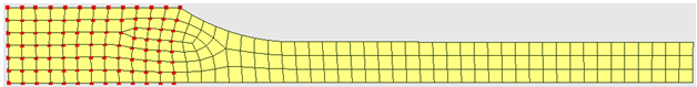
Create and Assign a Material
From the menu bar, select Model > Material.
Right-click in the material list and select Create New > Elasto-plastic > Johnson-Cook (2).
For Title, enter Aluminum. Enter all the material data
listed above.
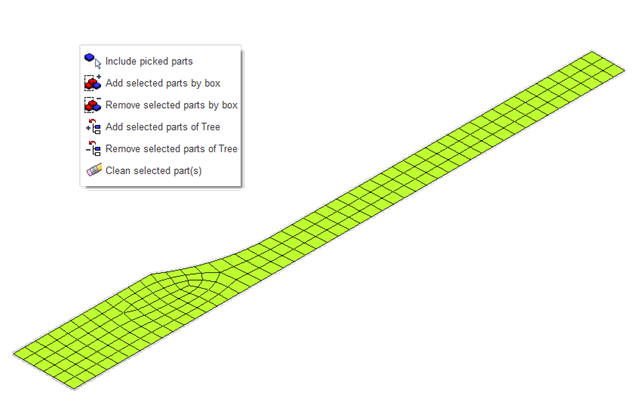
In the bottom of the material window, right-click in the
Support entry box and select Include
picked parts icon .
Figure 3.
Select the part in the modeling window
(left-click).
Right-click to validate the selection.
Press Enter or click Save > Close.
Create and Assign a Property
From the menu bar, select Model > Property.
Right-click in the property list and select Create New > Surface > Shell (1).
For Title, enter Pshell.
For Shell Thickness, enter 1.7.
In the bottom of the property window, right-click in the
Support entry box and select the Include
picked parts icon .
Select the part in the modeling window.
Right-click to validate the selection.
Click Save > Close.
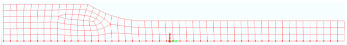
Define Boundary Conditions Representing Symmetry
From the menu bar, select LoadCase > Boundary Condition.
Right-click in the display list area and select Create
New.
For Name, enter constraint1 and click
Save.
Expand the folders Translation and Rotation.
Right-click in the Support entry box, click
Select in graphics and select the
Add/Remove nodes by picking selection icon to select the
nodes in the modeling window, as shown in the figure
below:
Figure 4.
Click Yes in the Dialog menu bar to validate your
selection.
To constrain the nodes, toggle Tx,
Ry and Rz and click
Save.
Repeat the same operations to create constraint2, as
shown in below:
Figure 5.
Toggle Tx, Ty,
Tz, Rx,
Ry and Rz, and click
Save.
Repeat the same operations to create constraint3, as
shown in below.
Press Shift, left-click and hold the mouse to draw a
box to select the nodes.
Figure 6.
Toggle Ty, Rx, and
Rz.
Click Save > Close.
Define Imposed Velocity
From the menu bar, select LoadCase > Imposed > Imposed Velocity.
Right-click in the display list area and select Create
New.
Set the Title to imposed_velocity.
Right-click in the entry box for Time function and
select Define Function.
A Function Window opens up.
For Function name, enter FUNC_VEL.
Enter the first point (0,1) and click
Validate.
Enter the second point (1e30,1) and click
Validate.
Click Save in the dialog.
Right-click in the Support entry box, click
Select in graphics and select the Add
nodes by box selection icon , to select the nodes in the modeling window, as shown in below:
Figure 7.
Go to the Properties tab and enter a Y-Scale factor =
-1.
Ensure Direction of the imposed velocity is set to X
(translation).
Click Save > Close.
Define a Time History Node
From the menu bar, select Data History > Time History.
In the list display area, right-click and select Create New > TH of nodes.
Enter the title Node_79.
Click Add Row to
add a new row.
With that row selected, scroll down to the input section and enter NODid as
79 and press Enter.
As an alternative, use the Pick button to select a node in the modeling window.
Click Save > Close.
Export the Model
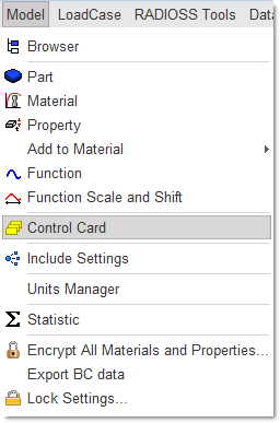
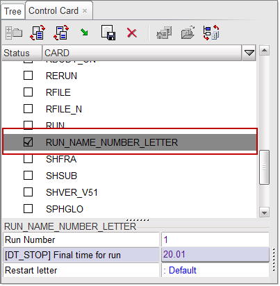
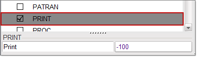
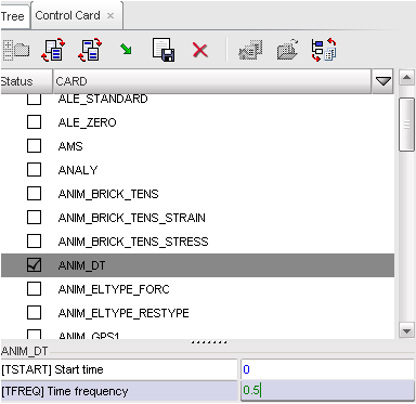
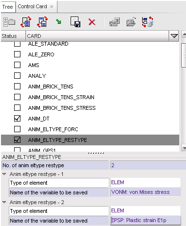
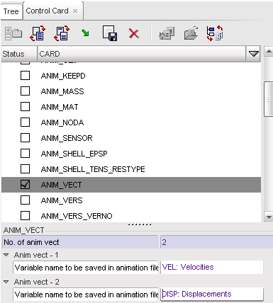
From the menu bar, select Model > Control Card:
Figure 8.
Enter the values for the Control Cards, as shown in the images below, saving
after every step:
Click File > Export > Radioss to export the solver file.
In the Write Block Format Radioss File window that
opens, navigate to your desired run directory and create a new folder named
TENSILE_TEST.
For filename, enter TENSILE and click
OK.
Leave the Header window empty and click on Save Model.
The file TENSILE_0000.rad is written.
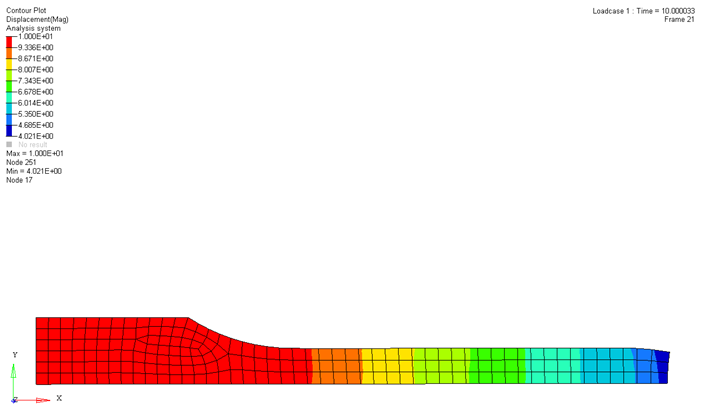
The model is now ready to run through the Starter and the Engine. It will produce
the result files TENSILEA* for animation in HyperView and TENSILE01 for time history
plotting in HyperGraph.
 .
.
 to select the
nodes in the modeling window, as shown in the figure
below:
to select the
nodes in the modeling window, as shown in the figure
below:
 , to select the nodes in the modeling window, as shown in below:
 to
add a new row.
to
add a new row.