RD-V: 0500 Shyue Shock Tube (JWL EOS)

A 1D shock tube filled with detonation gas products is used as a test model for the JWL Equation of state.
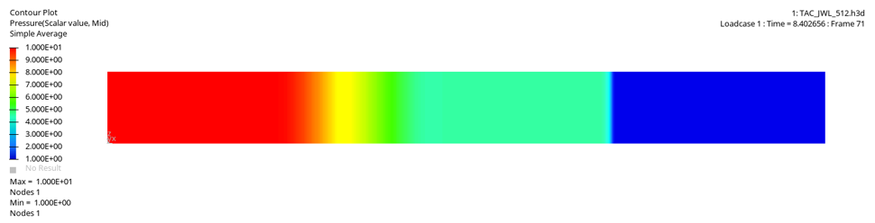


Figure 1.

The shock tube problem is a standard problem in gas dynamics. It can be used as a verification test as an exact solution exists. The Jones-Wilkins-Lee equation of state is used to model the behavior of detonation product of high explosives. Here a 1D shock tube case with detonation gas products governed by the Jones-Wilkins-Lee equation of state is built, and the results compared to the analytical solution. The influence of the second order integration scheme in time and space introduced with /ALE/MUSCL is shown.

The following criteria is used to compare the results:
  • Pressure
  • Mass density
  • Velocity
  • Specific energy

Options and Keywords Used

  • Explosive material, /MAT/LAW5 (JWL)
  • Multifluid law using the FVM solver, /MAT/LAW151 (MULTIFLUID)
  • Second order integration scheme, /ALE/MUSCL

Input Files

The input files used in this verification problem include:
  • <install_directory>/hwsolvers/demos/radioss/verification/Blast/0500_shyue_shock_tube/

Model Description

A shock tube consists in a long tube filled with gas, initially divided into two section separated by a diaphragm.

The gas in the two sections are in different physical states: there is usually a high-pressure and low-pressure section.

At the beginning of the experiment, the separation is removed and a compression shock runs into the low-pressure region, while a rarefaction wave moves into the high-pressure part of the tube. A contact discontinuity usually occurs between the two gases when the diaphragm is removed.

rad_ex_fig_13-3
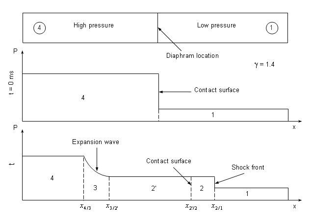
Figure 2. Schematic Shock Tube Problem with Pressure Distribution for Pre- and Post-diaphragm Removal

The interest of the shock tube problem is that it involves the three possible fundamental waves that can develop from uniform initial conditions: shock, rarefaction and contact waves.

Considered in one dimension, the shock tube is a Cartesian geometry Riemann problem, for which an analytical solution exists. When applied to a gas governed by a JWL equation of state, the shock tube case in 1D is called the test problem of Shyue. An analytical solution of this problem is described with analytical solutions available. 1

A shock tube 100 cm long is filled with detonation gas products and is divided of two chambers of equal length. The gas pressure in the left section (the high-pressure section) is 10 times the pressure in the right section (low-pressure section).

The physical properties of the detonation gas products in the right and left sections are:
Table 1. Initial Conditions
High Pressure Section Low Pressure Section
Pressure P 10.0 Mbar 1 Mbar
Mass density ρ 1.7 g c m 3 MathType@MTEF@5@5@+= feaahqart1ev3aqatCvAUfeBSjuyZL2yd9gzLbvyNv2CaerbuLwBLn hiov2DGi1BTfMBaeXatLxBI9gBaerbd9wDYLwzYbItLDharqqtubsr 4rNCHbGeaGqiVu0Je9sqqrpepC0xbbL8F4rqqrFfpeea0xe9Lq=Jc9 vqaqpepm0xbba9pwe9Q8fs0=yqaqpepae9pg0FirpepeKkFr0xfr=x fr=xb9adbaqaaeGaciGaaiaabeqaamaabaabaaGcbaWaaSaaaeaaca WGNbaabaGaam4yaiaad2gadaahaaWcbeqaaiaaiodaaaaaaaaa@39B4@ 1.0 g c m 3 MathType@MTEF@5@5@+= feaahqart1ev3aqatCvAUfeBSjuyZL2yd9gzLbvyNv2CaerbuLwBLn hiov2DGi1BTfMBaeXatLxBI9gBaerbd9wDYLwzYbItLDharqqtubsr 4rNCHbGeaGqiVu0Je9sqqrpepC0xbbL8F4rqqrFfpeea0xe9Lq=Jc9 vqaqpepm0xbba9pwe9Q8fs0=yqaqpepae9pg0FirpepeKkFr0xfr=x fr=xb9adbaqaaeGaciGaaiaabeqaamaabaabaaGcbaWaaSaaaeaaca WGNbaabaGaam4yaiaad2gadaahaaWcbeqaaiaaiodaaaaaaaaa@39B4@
Velocity u MathType@MTEF@5@5@+= feaagKart1ev2aaatCvAUfeBSjuyZL2yd9gzLbvyNv2CaerbuLwBLn hiov2DGi1BTfMBaeXatLxBI9gBaerbd9wDYLwzYbItLDharqqtubsr 4rNCHbGeaGqiVu0Je9sqqrpepC0xbbL8F4rqqrFfpeea0xe9Lq=Jc9 vqaqpepm0xbba9pwe9Q8fs0=yqaqpepae9pg0FirpepeKkFr0xfr=x fr=xb9adbaqaaeGaciGaaiaabeqaamaabaabaaGcbaGaamyDaaaa@36F0@ 0.0 c m μ s MathType@MTEF@5@5@+= feaahqart1ev3aqatCvAUfeBSjuyZL2yd9gzLbvyNv2CaerbuLwBLn hiov2DGi1BTfMBaeXatLxBI9gBaerbd9wDYLwzYbItLDharqqtubsr 4rNCHbGeaGqiVu0Je9sqqrpepC0xbbL8F4rqqrFfpeea0xe9Lq=Jc9 vqaqpepm0xbba9pwe9Q8fs0=yqaqpepae9pg0FirpepeKkFr0xfr=x fr=xb9adbaqaaeGaciGaaiaabeqaamaabaabaaGcbaWaaSaaaeaaca WGJbGaamyBaaqaaiabeY7aTjaadohaaaaaaa@3A8C@ 0.0 c m μ s MathType@MTEF@5@5@+= feaahqart1ev3aqatCvAUfeBSjuyZL2yd9gzLbvyNv2CaerbuLwBLn hiov2DGi1BTfMBaeXatLxBI9gBaerbd9wDYLwzYbItLDharqqtubsr 4rNCHbGeaGqiVu0Je9sqqrpepC0xbbL8F4rqqrFfpeea0xe9Lq=Jc9 vqaqpepm0xbba9pwe9Q8fs0=yqaqpepae9pg0FirpepeKkFr0xfr=x fr=xb9adbaqaaeGaciGaaiaabeqaamaabaabaaGcbaWaaSaaaeaaca WGJbGaamyBaaqaaiabeY7aTjaadohaaaaaaa@3A8C@

The following system is used: cm, ms, g, daN, Mbar

Model Method

Each section is modeled by one component.

Both are meshed with 3D /BRICK elements. As the problem is one-dimensional, the relevant mesh size is the width of the mesh in the direction of interest (here, the direction of propagation of the compression and rarefaction waves). The size of the mesh in the other directions is of no importance (Figure 3).


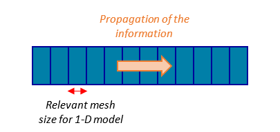
Figure 3. Relevant Mesh Size for 1D Model
The model is meshed with 512 elements (which accounts for a mesh size in the direction of interest of roughly 2 mm).


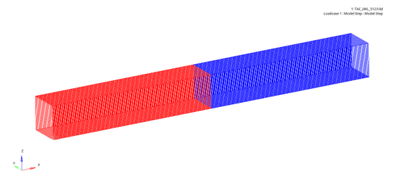
Figure 4. Mesh Used for the 1D Shock Tube

The detonation gas products in the two sections are modeled using /MAT/JWL which is based on the JWL equation of state. The JWL materials are then referenced by /MAT/MULTIFLUID which allows the use of the Radioss finite volume solver.

The two material laws (/MAT/JWL) that represent the high- and low-pressure gas are used in a multifluid law (/MAT/MULTILFUID) in order to use the Finite Volume solver.

Detonation Gas Products Modeling

This shock tube case considers detonation gas products. In Radioss, explosive materials defined with /MAT/JWL are considered solid until they detonate. To get these materials in their gaseous states, a detonator is created with a /DFS/DETPOINT card. The detonation time variable TDET is set to -1E30s (meaning minus infinity), ensuring that at the beginning at the simulation all the explosive material in the model consists of detonation gas products.

Detonation gas product behavior is governed by the JWL equation of state. This EOS relates Pressure to the specific volume of the explosive.

The JWL EOS expression is:(1) P jwl υ,E =A 1 ω R 1 υ e R 1 υ +B 1 ω R 2 υ e R 2 υ + ωE υ MathType@MTEF@5@5@+= feaahqart1ev3aqatCvAUfeBSjuyZL2yd9gzLbvyNv2CaerbuLwBLn hiov2DGi1BTfMBaeXatLxBI9gBaerbd9wDYLwzYbItLDharqqtubsr 4rNCHbGeaGqiVu0Je9sqqrpepC0xbbL8F4rqqrFfpeea0xe9Lq=Jc9 vqaqpepm0xbbG8FasPYRqj0=yi0dXdbba9pGe9xq=JbbG8A8frFve9 Fve9Ff0dmeaabaqaciGacaGaaeqabaWaaeaaeaaakeaaqaaaaaaaaa WdbiaadcfapaWaaSbaaSqaa8qacaWGQbGaam4DaiaadYgaa8aabeaa k8qadaqadaWdaeaapeGaeqyXduNaaiilaiaadweaaiaawIcacaGLPa aacqGH9aqpcaWGbbWaaeWaa8aabaWdbiaaigdacqGHsisldaWcaaWd aeaapeGaeqyYdChapaqaa8qacaWGsbWdamaaBaaaleaapeGaaGymaa WdaeqaaOWdbiabew8a1baaaiaawIcacaGLPaaacaWGLbWdamaaCaaa leqabaWdbiabgkHiTiaadkfapaWaaSbaaWqaa8qacaaIXaaapaqaba WcpeGaeqyXduhaaOGaey4kaSIaamOqamaabmaapaqaa8qacaaIXaGa eyOeI0YaaSaaa8aabaWdbiabeM8a3bWdaeaapeGaamOua8aadaWgaa WcbaWdbiaaikdaa8aabeaak8qacqaHfpqDaaaacaGLOaGaayzkaaGa amyza8aadaahaaWcbeqaa8qacqGHsislcaWGsbWdamaaBaaameaape GaaGOmaaWdaeqaaSWdbiabew8a1baakiabgUcaRmaalaaapaqaa8qa cqaHjpWDcaWGfbaapaqaa8qacqaHfpqDaaaaaa@66F7@
Where,
P jwl MathType@MTEF@5@5@+= feaahqart1ev3aqatCvAUfeBSjuyZL2yd9gzLbvyNv2CaerbuLwBLn hiov2DGi1BTfMBaeXatLxBI9gBaerbd9wDYLwzYbItLDharqqtubsr 4rNCHbGeaGqiVu0Je9sqqrpepC0xbbL8F4rqqrFfpeea0xe9Lq=Jc9 vqaqpepm0xbbG8FasPYRqj0=yi0dXdbba9pGe9xq=JbbG8A8frFve9 Fve9Ff0dmeaabaqaciGacaGaaeqabaWaaeaaeaaakeaaqaaaaaaaaa WdbiaadcfapaWaaSbaaSqaa8qacaWGQbGaam4DaiaadYgaa8aabeaa aaa@3A87@
Pressure
υ MathType@MTEF@5@5@+= feaahqart1ev3aqatCvAUfeBSjuyZL2yd9gzLbvyNv2CaerbuLwBLn hiov2DGi1BTfMBaeXatLxBI9gBaerbd9wDYLwzYbItLDharqqtubsr 4rNCHbGeaGqiVu0Je9sqqrpepC0xbbL8F4rqqrFfpeea0xe9Lq=Jc9 vqaqpepm0xbbG8FasPYRqj0=yi0dXdbba9pGe9xq=JbbG8A8frFve9 Fve9Ff0dmeaabaqaciGacaGaaeqabaWaaeaaeaaakeaaqaaaaaaaaa Wdbiabew8a1baa@3843@
Relative volume υ= ρ 0 ρ MathType@MTEF@5@5@+= feaahqart1ev3aqatCvAUfeBSjuyZL2yd9gzLbvyNv2CaerbuLwBLn hiov2DGi1BTfMBaeXatLxBI9gBaerbd9wDYLwzYbItLDharqqtubsr 4rNCHbGeaGqiVCI8FfYJH8YrFfeuY=Hhbbf9v8qqaqFr0xc9pk0xbb a9q8WqFfeaY=biLkVcLq=JHqpepeea0=as0Fb9pgeaYRXxe9vr0=vr 0=vqpWqaaeaabiGaciaacaqabeaadaqaaqaaaOqaaabaaaaaaaaape GaeqyXduNaeyypa0ZaaSaaa8aabaWdbiabeg8aY9aadaWgaaWcbaWd biaaicdaa8aabeaaaOqaa8qacqaHbpGCaaaaaa@3DB3@
A MathType@MTEF@5@5@+= feaagKart1ev2aaatCvAUfeBSjuyZL2yd9gzLbvyNv2CaerbuLwBLn hiov2DGi1BTfMBaeXatLxBI9gBaerbd9wDYLwzYbItLDharqqtubsr 4rNCHbGeaGqiVu0Je9sqqrpepC0xbbL8F4rqqrFfpeea0xe9Lq=Jc9 vqaqpepm0xbba9pwe9Q8fs0=yqaqpepae9pg0FirpepeKkFr0xfr=x fr=xb9adbaqaaeGaciGaaiaabeqaamaabaabaaGcbaGaamyraaaa@36C0@ , B MathType@MTEF@5@5@+= feaagKart1ev2aaatCvAUfeBSjuyZL2yd9gzLbvyNv2CaerbuLwBLn hiov2DGi1BTfMBaeXatLxBI9gBaerbd9wDYLwzYbItLDharqqtubsr 4rNCHbGeaGqiVu0Je9sqqrpepC0xbbL8F4rqqrFfpeea0xe9Lq=Jc9 vqaqpepm0xbba9pwe9Q8fs0=yqaqpepae9pg0FirpepeKkFr0xfr=x fr=xb9adbaqaaeGaciGaaiaabeqaamaabaabaaGcbaGaamyraaaa@36C0@ , R 1 MathType@MTEF@5@5@+= feaahqart1ev3aqatCvAUfeBSjuyZL2yd9gzLbvyNv2CaerbuLwBLn hiov2DGi1BTfMBaeXatLxBI9gBaerbd9wDYLwzYbItLDharqqtubsr 4rNCHbGeaGqiVu0Je9sqqrpepC0xbbL8F4rqqrFfpeea0xe9Lq=Jc9 vqaqpepm0xbbG8FasPYRqj0=yi0dXdbba9pGe9xq=JbbG8A8frFve9 Fve9Ff0dmeaabaqaciGacaGaaeqabaWaaeaaeaaakeaaqaaaaaaaaa WdbiaadkfapaWaaSbaaSqaa8qacaaIXaaapaqabaaaaa@3868@ , R 2 MathType@MTEF@5@5@+= feaahqart1ev3aqatCvAUfeBSjuyZL2yd9gzLbvyNv2CaerbuLwBLn hiov2DGi1BTfMBaeXatLxBI9gBaerbd9wDYLwzYbItLDharqqtubsr 4rNCHbGeaGqiVu0Je9sqqrpepC0xbbL8F4rqqrFfpeea0xe9Lq=Jc9 vqaqpepm0xbbG8FasPYRqj0=yi0dXdbba9pGe9xq=JbbG8A8frFve9 Fve9Ff0dmeaabaqaciGacaGaaeqabaWaaeaaeaaakeaaqaaaaaaaaa WdbiaadkfapaWaaSbaaSqaa8qacaaIXaaapaqabaaaaa@3868@
Parameters specific to the explosives
ω
Gruneisen coefficient
E MathType@MTEF@5@5@+= feaagKart1ev2aaatCvAUfeBSjuyZL2yd9gzLbvyNv2CaerbuLwBLn hiov2DGi1BTfMBaeXatLxBI9gBaerbd9wDYLwzYbItLDharqqtubsr 4rNCHbGeaGqiVu0Je9sqqrpepC0xbbL8F4rqqrFfpeea0xe9Lq=Jc9 vqaqpepm0xbba9pwe9Q8fs0=yqaqpepae9pg0FirpepeKkFr0xfr=x fr=xb9adbaqaaeGaciGaaiaabeqaamaabaabaaGcbaGaamyraaaa@36C0@
Detonation energy per unit volume
The /MAT/JWL cards used for the detonation gas products are defined using the following parameters:
Table 2. Values of Input Parameters for the /MAT/JWL Cards
High Pressure Section Low Pressure Section
Density Initial density ρ 1.7 g c m 3 MathType@MTEF@5@5@+= feaahqart1ev3aqatCvAUfeBSjuyZL2yd9gzLbvyNv2CaerbuLwBLn hiov2DGi1BTfMBaeXatLxBI9gBaerbd9wDYLwzYbItLDharqqtubsr 4rNCHbGeaGqiVu0Je9sqqrpepC0xbbL8F4rqqrFfpeea0xe9Lq=Jc9 vqaqpepm0xbba9pwe9Q8fs0=yqaqpepae9pg0FirpepeKkFr0xfr=x fr=xb9adbaqaaeGaciGaaiaabeqaamaabaabaaGcbaWaaSaaaeaaca WGNbaabaGaam4yaiaad2gadaahaaWcbeqaaiaaiodaaaaaaaaa@39B4@ 1.0 g c m 3 MathType@MTEF@5@5@+= feaahqart1ev3aqatCvAUfeBSjuyZL2yd9gzLbvyNv2CaerbuLwBLn hiov2DGi1BTfMBaeXatLxBI9gBaerbd9wDYLwzYbItLDharqqtubsr 4rNCHbGeaGqiVu0Je9sqqrpepC0xbbL8F4rqqrFfpeea0xe9Lq=Jc9 vqaqpepm0xbba9pwe9Q8fs0=yqaqpepae9pg0FirpepeKkFr0xfr=x fr=xb9adbaqaaeGaciGaaiaabeqaamaabaabaaGcbaWaaSaaaeaaca WGNbaabaGaam4yaiaad2gadaahaaWcbeqaaiaaiodaaaaaaaaa@39B4@
Reference density ρ 0 1.84 g c m 3 MathType@MTEF@5@5@+= feaahqart1ev3aqatCvAUfeBSjuyZL2yd9gzLbvyNv2CaerbuLwBLn hiov2DGi1BTfMBaeXatLxBI9gBaerbd9wDYLwzYbItLDharqqtubsr 4rNCHbGeaGqiVu0Je9sqqrpepC0xbbL8F4rqqrFfpeea0xe9Lq=Jc9 vqaqpepm0xbba9pwe9Q8fs0=yqaqpepae9pg0FirpepeKkFr0xfr=x fr=xb9adbaqaaeGaciGaaiaabeqaamaabaabaaGcbaWaaSaaaeaaca WGNbaabaGaam4yaiaad2gadaahaaWcbeqaaiaaiodaaaaaaaaa@39B4@ 1.84 g c m 3 MathType@MTEF@5@5@+= feaahqart1ev3aqatCvAUfeBSjuyZL2yd9gzLbvyNv2CaerbuLwBLn hiov2DGi1BTfMBaeXatLxBI9gBaerbd9wDYLwzYbItLDharqqtubsr 4rNCHbGeaGqiVu0Je9sqqrpepC0xbbL8F4rqqrFfpeea0xe9Lq=Jc9 vqaqpepm0xbba9pwe9Q8fs0=yqaqpepae9pg0FirpepeKkFr0xfr=x fr=xb9adbaqaaeGaciGaaiaabeqaamaabaabaaGcbaWaaSaaaeaaca WGNbaabaGaam4yaiaad2gadaahaaWcbeqaaiaaiodaaaaaaaaa@39B4@
JWL parameters A 8.545 Mbar
B 0.205 Mbar
R1 4.6
R2 1.35
ω 0.25
Chapman-Jouguet parameters Detonation velocity DCJ 0.693 c m μ s MathType@MTEF@5@5@+= feaahqart1ev3aqatCvAUfeBSjuyZL2yd9gzLbvyNv2CaerbuLwBLn hiov2DGi1BTfMBaeXatLxBI9gBaerbd9wDYLwzYbItLDharqqtubsr 4rNCHbGeaGqiVu0Je9sqqrpepC0xbbL8F4rqqrFfpeea0xe9Lq=Jc9 vqaqpepm0xbba9pwe9Q8fs0=yqaqpepae9pg0FirpepeKkFr0xfr=x fr=xb9adbaqaaeGaciGaaiaabeqaamaabaabaaGcbaWaaSaaaeaaca WGJbGaamyBaaqaaiabeY7aTjaadohaaaaaaa@3A8C@
Detonation pressure PCJ 0.21 Mbar
Detonation Energy E0 42.88164777 Mbar 7.233944805 Mbar
The initial density corresponds to the density of the explosive in each compartment, while the reference density is the one used to compute the relative volume used in the JWL equation of state, as:(2) υ = ρ 0 ρ MathType@MTEF@5@5@+= feaahqart1ev3aqatCvAUfeBSjuyZL2yd9gzLbvyNv2CaerbuLwBLn hiov2DGi1BTfMBaeXatLxBI9gBaerbd9wDYLwzYbItLDharqqtubsr 4rNCHbGeaGqiVCI8FfYJH8YrFfeuY=Hhbbf9v8qqaqFr0xc9pk0xbb a9q8WqFfeaY=biLkVcLq=JHqpepeea0=as0Fb9pgeaYRXxe9vr0=vr 0=vqpWqaaeaabiGaciaacaqabeaadaqaaqaaaOqaaabaaaaaaaaape GaeqyXduNaeyypa0ZaaSaaa8aabaWdbiabeg8aY9aadaWgaaWcbaWd biaaicdaa8aabeaaaOqaa8qacqaHbpGCaaaaaa@3DB3@

The JWL parameters comes from the reference article. As this model is a test case for computer code verification, they are not related to any existing explosive materials.

The Chapman-Jouguet parameters used for modelling the propagation of the detonation are of no importance as this model only considers gaseous materials. The Chapman-Jouguet parameters of the TNT have been used for detonation pressure PCJ and velocity DCJ. The precise value of these two parameters has no influence on the results, as they are only used to model the detonation process of the solid explosive. The detonation energy E0 is computed using the JWL equation of state expression to get an initial pressure P l e f t = 10 M b a r MathType@MTEF@5@5@+= feaagKart1ev2aaatCvAUfeBSjuyZL2yd9gzLbvyNv2CaerbuLwBLn hiov2DGi1BTfMBaeXatLxBI9gBaerbd9wDYLwzYbItLDharqqtubsr 4rNCHbGeaGqiVu0Je9sqqrpepC0xbbL8F4rqqrFfpeea0xe9Lq=Jc9 vqaqpepm0xbba9pwe9Q8fs0=yqaqpepae9pg0FirpepeKkFr0xfr=x fr=xb9adbaqaaeGaciGaaiaabeqaamaabaabaaGcbaGaamiuamaaBa aaleaacaWGSbGaamyzaiaadAgacaWG0baabeaakiabg2da9iaaigda caaIWaGaaGPaVlaad2eacaWGIbGaamyyaiaadkhaaaa@425C@ for the high-pressure gas, and P r i g h t = 1 M b a r MathType@MTEF@5@5@+= feaagKart1ev2aaatCvAUfeBSjuyZL2yd9gzLbvyNv2CaerbuLwBLn hiov2DGi1BTfMBaeXatLxBI9gBaerbd9wDYLwzYbItLDharqqtubsr 4rNCHbGeaGqiVu0Je9sqqrpepC0xbbL8F4rqqrFfpeea0xe9Lq=Jc9 vqaqpepm0xbba9pwe9Q8fs0=yqaqpepae9pg0FirpepeKkFr0xfr=x fr=xb9adbaqaaeGaciGaaiaabeqaamaabaabaaGcbaGaamiuamaaBa aaleaacaWGYbGaamyAaiaadEgacaWGObGaamiDaaqabaGccqGH9aqp caaIXaGaaGPaVlaad2eacaWGIbGaamyyaiaadkhaaaa@429A@ for the low-pressure gas.

Two instances of the multimaterial law (/MAT/MULTILFUID) are created, each one corresponding to a section and integrating the gas defined using LAW5, with a volumetric fraction of 1.

/EULER/MAT should be defined for the /MAT/MULTIFLUID materials, to indicate that they are EULERIAN materials.

The /ALE/MUSCL option activates a full second order integration scheme in time and space, which increases the accuracy of the results. The results of the simulations with and without /ALE/MUSCL will be compared to the analytical solution. 1

Boundary Conditions

Boundary conditions around the 1D shock tube are sliding walls, which is the default when using (/MAT/MULTIFLUID).


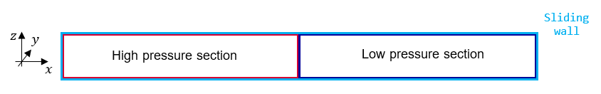
Figure 5. Boundary Conditions for the Shock Tube

Engine Control

Since Radioss 2019.0 release, the time step scale factor for all ALE and EULER elements is set by default to 0.5.

It can be modified using the keyword /DT/ALE:
/DT/ALE
0.5                  0.000000

Results

Results are examined 12 μ s after the removal of the separation between the two chambers.
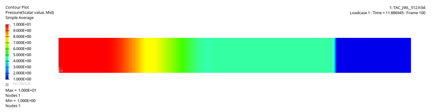


Figure 6. Pressure Contour after 12 μ s

Spatial profile of pressure, mass density, velocity and energy are compared to the analytical results given in the reference article. These profiles are obtained by drawing a node path along the tube. To draw node paths, the elemental results visible on the animation have to be averaged at the nodes, using for example the averaging method simple.

Profiles of pressure and mass density along the tube after 12 μ s are visible on Figure 7 and Figure 8, as well as similar profiles for velocity and specific energy on Figure 9 and Figure 10, with the curve obtained from the analytical solution.
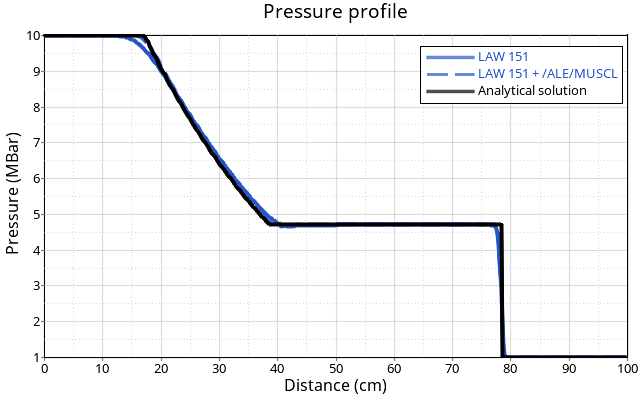
Figure 7. Pressure Profile. (with and without /ALE/MUSCL, compared to analytical solution)


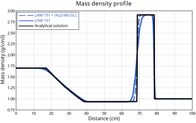
Figure 8. Mass Density Profile. (with and without /ALE/MUSCL, compared to analytical solution)


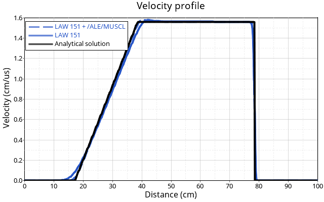
Figure 9. Velocity Profile. (with and without /ALE/MUSCL, compared to analytical solution)


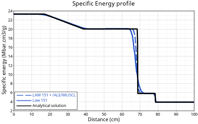
Figure 10. Specific Energy Profile. (with and without /ALE/MUSCL, compared to analytical solution)

The simulation results for these four variables matches closely the analytical solution, and the fit is better for the results obtained with /ALE/MUSCL enabled.

The difference between numerical results and the analytical solution can be quantified by computing the £2-norm error between the curves.

The £2-norm error (also named Eulerian norm error) between a numerical result Y n u m MathType@MTEF@5@5@+= feaagKart1ev2aaatCvAUfeBSjuyZL2yd9gzLbvyNv2CaerbuLwBLn hiov2DGi1BTfMBaeXatLxBI9gBaerbd9wDYLwzYbItLDharqqtubsr 4rNCHbGeaGqiVu0Je9sqqrpepC0xbbL8F4rqqrFfpeea0xe9Lq=Jc9 vqaqpepm0xbba9pwe9Q8fs0=yqaqpepae9pg0FirpepeKkFr0xfr=x fr=xb9adbaqaaeGaciGaaiaabeqaamaabaabaaGcbaGaamywamaaBa aaleaacaWGUbGaamyDaiaad2gaaeqaaaaa@39DF@ and the exact solution Y e x a c t MathType@MTEF@5@5@+= feaagKart1ev2aaatCvAUfeBSjuyZL2yd9gzLbvyNv2CaerbuLwBLn hiov2DGi1BTfMBaeXatLxBI9gBaerbd9wDYLwzYbItLDharqqtubsr 4rNCHbGeaGqiVu0Je9sqqrpepC0xbbL8F4rqqrFfpeea0xe9Lq=Jc9 vqaqpepm0xbba9pwe9Q8fs0=yqaqpepae9pg0FirpepeKkFr0xfr=x fr=xb9adbaqaaeGaciGaaiaabeqaamaabaabaaGcbaGaamywamaaBa aaleaacaWGLbGaamiEaiaadggacaWGJbGaamiDaaqabaaaaa@3BAE@ is defined as:(3) L 2  error = ( Y num Y exact ) 2 dx Y exact 2 dx MathType@MTEF@5@5@+= feaahqart1ev3aqatCvAUfeBSjuyZL2yd9gzLbvyNv2CaerbuLwBLn hiov2DGi1BTfMBaeXatLxBI9gBaerbd9wDYLwzYbItLDharqqtubsr 4rNCHbGeaGqiVu0Je9sqqrpepC0xbbL8F4rqqrFfpeea0xe9Lq=Jc9 vqaqpepm0xbbG8FasPYRqj0=yi0dXdbba9pGe9xq=JbbG8A8frFve9 Fve9Ff0dmeaabaqaciGacaGaaeqabaWaaeaaeaaakeaatuuDJXwAK1 uy0HwmaeHbfv3ySLgzG0uy0Hgip5wzaGqbbabaaaaaaaaapeGae8Ne HW0damaaBaaaleaapeGaaGOmaaWdaeqaaOWdbiaacckacaWGLbGaam OCaiaadkhacaWGVbGaamOCaiaacckacqGH9aqpdaGcaaWdaeaapeWa aSaaa8aabaWdbmaapeaabaGaaiikaiaadMfapaWaaSbaaSqaa8qaca WGUbGaamyDaiaad2gaa8aabeaak8qacqGHsislcaWGzbWdamaaBaaa leaapeGaamyzaiaadIhacaWGHbGaam4yaiaadshaa8aabeaak8qaca GGPaWdamaaCaaaleqabaWdbiaaikdaaaGccaWGKbGaamiEaaWcbeqa b0Gaey4kIipaaOWdaeaapeWaa8qaaeaacaWGzbWdamaaDaaaleaape GaamyzaiaadIhacaWGHbGaam4yaiaadshaa8aabaWdbiaaikdaaaGc caWGKbGaamiEaaWcbeqab0Gaey4kIipaaaaaleqaaaaa@66E6@
The £2-norm error to the analytical solution on pressure, mass density, velocity are:
Table 3. £2-norm error to the analytical solution with and without /ALE/MUSCL
  /ALE/MUSCL Pressure Mass Density Velocity Specific Energy
£2-norm

relative error

enabled 2.0% 6.5% 3.9% 4.5%
disabled 2.5% 9.2% 4.7% 6.7%

As shown on Table 3, the use of /ALE/MUSCL allows for better precision in the numerical results.

Conclusion

The numerical results show a good correlation with the analytical solution presented in the reference article. /MAT/JWL used within a /MAT/MULTIFLUID multi-material law allows for an accurate resolution use of the JWL equation of state.

There are clear benefits of using /ALE/MUSCL in term of precision.

1 Kamm, J.R. An Exact, Compressible One-Dimensional Riemann Solver for General, Convex Equation of State. Los Alamos National Laboratory, 2015