RD-V: 0520 Double Oblique Shock

A supersonic flow encounters two successive wedges and oblique shock are formed.


Figure 1.

The double oblique shock is a classic example in compressible fluid mechanics. It involves a supersonic flow propagating along a wall with two unequal wedges. Each wedge slows down and compresses the flow with the formation of a shock wave. These two shocks then merge into a stronger, single one away from the wall, and a contact wave is formed inside the flow between the shocked states. The numerical results obtained for the thermodynamics quantities in each state of the flow can be compared to analytical values obtained with compressible fluid mechanics theory.

Options and Keywords Used

Input Files

The input file used in this verification problem includes:
  • <install_directory>/hwsolvers/demos/radioss/verification/Blast/0520_double_shock/*
Note: The keywords not supported by HyperMesh are in a separate include file. To view the file in HyperMesh, it is recommended to import the file using the “Include File: Skip” option.

Model Description

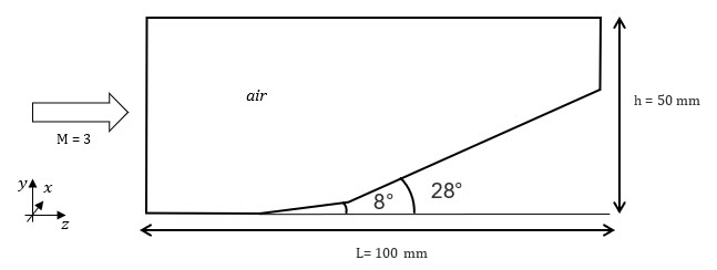
A supersonic wind tunnel (100mm length, 50 mm height) is filled with a supersonic flow Machine number (M=3) of air.

The lower wall includes two wedges of 8 degrees and 28 degrees.

The two wedges slow the flow down with the formation of shock waves.


Figure 2. Problem Description for Double Oblique Shock

Units: mm, ms, g, N, MPa

Model Method

The fluid domain is meshed with 2D quads elements with an average mesh size of 0.15*0.15 mm. This accounts for around 160,000 elements.

The material law used for air is a hydrodynamic fluid (/MAT/LAW6) in combination with an ideal gas equation of state (/EOS/IDEAL-GAS).

The hydrodynamic fluid (/MAT/LAW6) is used within a multifluid law (/MAT/MULTILFUID) which uses a Finite Volume solver. The fluid is considered non-viscous.

Air is defined with the following characteristics:
/MAT/LAW6
Initial density
1.225E-6 g m m 3 MathType@MTEF@5@5@+= feaagKart1ev2aqatCvAUfeBSjuyZL2yd9gzLbvyNv2CaerbuLwBLn hiov2DGi1BTfMBaeXatLxBI9gBaerbd9wDYLwzYbItLDharqqtubsr 4rNCHbGeaGqiVu0Je9sqqrpepC0xbbL8F4rqGqFfpeea0xe9vq=Jb9 vqpeea0xd9q8qiYRWxGi6xij=hbba9q8aq0=yq=He9q8qiLsFr0=vr 0=vr0db8meaabaqaciGacaGaaeqabaWaaeaaeaaakeaadaWcaaqaai aacEgaaeaacaGGTbGaaiyBamaaCaaaleqabaGaai4maaaaaaaaaa@3B29@
/EOS/IDEAL-GAS
Heat capacity ratio
1.4
Initial pressure
0.1 MPa
Initial density
1.225E-6 g m m 3 MathType@MTEF@5@5@+= feaagKart1ev2aqatCvAUfeBSjuyZL2yd9gzLbvyNv2CaerbuLwBLn hiov2DGi1BTfMBaeXatLxBI9gBaerbd9wDYLwzYbItLDharqqtubsr 4rNCHbGeaGqiVu0Je9sqqrpepC0xbbL8F4rqGqFfpeea0xe9vq=Jb9 vqpeea0xd9q8qiYRWxGi6xij=hbba9q8aq0=yq=He9q8qiLsFr0=vr 0=vr0db8meaabaqaciGacaGaaeqabaWaaeaaeaaakeaadaWcaaqaai aacEgaaeaacaGGTbGaaiyBamaaCaaaleqabaGaai4maaaaaaaaaa@3B29@

Since there is only one fluid (air), the multi-material law only integrates the air defined using LAW6, with a volumer fraction of 1.

To indicate that it is an EULERIAN material, /EULER/MAT should be defined for the /MAT/MULTIFLUID material.

The /ALE/MUSCL option activates a full second order integration scheme in time and space. It should be added for more precision.
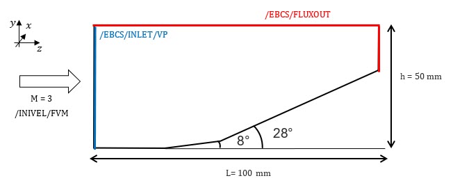
Boundary Conditions


Figure 3. Boundary Condition for Double Oblique Shock
The fluid is given an initial velocity along the z-axis, defined with /INIVEL/FVM as:(1) V x = 0 m s MathType@MTEF@5@5@+= feaagKart1ev2aqatCvAUfeBSjuyZL2yd9gzLbvyNv2CaerbuLwBLn hiov2DGi1BTfMBaeXatLxBI9gBaerbd9wDYLwzYbItLDharqqtubsr 4rNCHbGeaGqiVu0Je9sqqrpepC0xbbL8F4rqGqFfpeea0xe9vq=Jb9 vqpeea0xd9q8qiYRWxGi6xij=hbba9q8aq0=yq=He9q8qiLsFr0=vr 0=vr0db8meaabaqaciGacaGaaeqabaWaaeaaeaaakeaacaWGwbWaaS baaSqaaiaadIhaaeqaaOGaeyypa0JaaGimamaalaaabaGaaiyBaaqa aiaacohaaaaaaa@3D2E@ (2) V y = 0 m s MathType@MTEF@5@5@+= feaagKart1ev2aqatCvAUfeBSjuyZL2yd9gzLbvyNv2CaerbuLwBLn hiov2DGi1BTfMBaeXatLxBI9gBaerbd9wDYLwzYbItLDharqqtubsr 4rNCHbGeaGqiVu0Je9sqqrpepC0xbbL8F4rqGqFfpeea0xe9vq=Jb9 vqpeea0xd9q8qiYRWxGi6xij=hbba9q8aq0=yq=He9q8qiLsFr0=vr 0=vr0db8meaabaqaciGacaGaaeqabaWaaeaaeaaakeaacaWGwbWaaS baaSqaaiaadIhaaeqaaOGaeyypa0JaaGimamaalaaabaGaaiyBaaqa aiaacohaaaaaaa@3D2E@ (3) V z = 1014 .18510 m s MathType@MTEF@5@5@+= feaagKart1ev2aqatCvAUfeBSjuyZL2yd9gzLbvyNv2CaerbuLwBLn hiov2DGi1BTfMBaeXatLxBI9gBaerbd9wDYLwzYbItLDharqqtubsr 4rNCHbGeaGqiVu0Je9sqqrpepC0xbbL8F4rqGqFfpeea0xe9vq=Jb9 vqpeea0xd9q8qiYRWxGi6xij=hbba9q8aq0=yq=He9q8qiLsFr0=vr 0=vr0db8meaabaqaciGacaGaaeqabaWaaeaaeaaakeaacaWGwbWaaS baaSqaaiaadQhaaeqaaOGaeyypa0deaaaaaaaaa8qacaqGXaGaaeim aiaabgdacaqG0aGaaeOlaiaabgdacaqG4aGaaeynaiaabgdacaqGWa WdamaalaaabaGaaiyBaaqaaiaacohaaaaaaa@43B6@
The value of velocity V z MathType@MTEF@5@5@+= feaagKart1ev2aqatCvAUfeBSjuyZL2yd9gzLbvyNv2CaerbuLwBLn hiov2DGi1BTfMBaeXatLxBI9gBaerbd9wDYLwzYbItLDharqqtubsr 4rNCHbGeaGqiVu0Je9sqqrpepC0xbbL8F4rqGqFfpeea0xe9vq=Jb9 vqpeea0xd9q8qiYRWxGi6xij=hbba9q8aq0=yq=He9q8qiLsFr0=vr 0=vr0db8meaabaqaciGacaGaaeqabaWaaeaaeaaakeaacaWGwbWaaS baaSqaaiaadQhaaeqaaaaa@396E@ corresponds to a speed of Mach 3, with the Mach number M MathType@MTEF@5@5@+= feaagKart1ev2aqatCvAUfeBSjuyZL2yd9gzLbvyNv2CaerbuLwBLn hiov2DGi1BTfMBaeXatLxBI9gBaerbd9wDYLwzYbItLDharqqtubsr 4rNCHbGeaGqiVu0Je9sqqrpepC0xbbL8F4rqGqFfpeea0xe9vq=Jb9 vqpeea0xd9q8qiYRWxGi6xij=hbba9q8aq0=yq=He9q8qiLsFr0=vr 0=vr0db8meaabaqaciGacaGaaeqabaWaaeaaeaaakeaacaWGnbaaaa@383A@ defined as:(4) M = V z a MathType@MTEF@5@5@+= feaagKart1ev2aqatCvAUfeBSjuyZL2yd9gzLbvyNv2CaerbuLwBLn hiov2DGi1BTfMBaeXatLxBI9gBaerbd9wDYLwzYbItLDharqqtubsr 4rNCHbGeaGqiVu0Je9sqqrpepC0xbbL8F4rqGqFfpeea0xe9vq=Jb9 vqpeea0xd9q8qiYRWxGi6xij=hbba9q8aq0=yq=He9q8qiLsFr0=vr 0=vr0db8meaabaqaciGacaGaaeqabaWaaeaaeaaakeaacaWGnbGaey ypa0ZaaSaaaeaacaWGwbWaaSbaaSqaaiaadQhaaeqaaaGcbaGaamyy aaaaaaa@3C46@
Where, a MathType@MTEF@5@5@+= feaagKart1ev2aqatCvAUfeBSjuyZL2yd9gzLbvyNv2CaerbuLwBLn hiov2DGi1BTfMBaeXatLxBI9gBaerbd9wDYLwzYbItLDharqqtubsr 4rNCHbGeaGqiVu0Je9sqqrpepC0xbbL8F4rqGqFfpeea0xe9vq=Jb9 vqpeea0xd9q8qiYRWxGi6xij=hbba9q8aq0=yq=He9q8qiLsFr0=vr 0=vr0db8meaabaqaciGacaGaaeqabaWaaeaaeaaakeaacaWGHbaaaa@384E@ is the sound velocity, which is computed as:(5) a = γ P ρ MathType@MTEF@5@5@+= feaagKart1ev2aqatCvAUfeBSjuyZL2yd9gzLbvyNv2CaerbuLwBLn hiov2DGi1BTfMBaeXatLxBI9gBaerbd9wDYLwzYbItLDharqqtubsr 4rNCHbGeaGqiVu0Je9sqqrpepC0xbbL8F4rqGqFfpeea0xe9vq=Jb9 vqpeea0xd9q8qiYRWxGi6xij=hbba9q8aq0=yq=He9q8qiLsFr0=vr 0=vr0db8meaabaqaciGacaGaaeqabaWaaeaaeaaakeaacaWGHbGaey ypa0ZaaOaaaeaadaWcaaqaaiabeo7aNjaadcfaaeaacqaHbpGCaaaa leqaaaaa@3DBB@ (6) a = 338 m s MathType@MTEF@5@5@+= feaagKart1ev2aqatCvAUfeBSjuyZL2yd9gzLbvyNv2CaerbuLwBLn hiov2DGi1BTfMBaeXatLxBI9gBaerbd9wDYLwzYbItLDharqqtubsr 4rNCHbGeaGqiVu0Je9sqqrpepC0xbbL8F4rqGqFfpeea0xe9vq=Jb9 vqpeea0xd9q8qiYRWxGi6xij=hbba9q8aq0=yq=He9q8qiLsFr0=vr 0=vr0db8meaabaqaciGacaGaaeqabaWaaeaaeaaakeaacaWGHbGaey ypa0JaaG4maiaaiodacaaI4aWaaSaaaeaacaGGTbaabaGaai4Caaaa aaa@3D88@

When using /MAT/MULTIFLUID, the default boundary conditions are sliding walls.

A non-reflecting inlet is defined using /EBCS/INLET/VP. Input density and pressure are defined for the air in the multi-material law.

A non-reflecting boundary is defined with /EBCS/FLUXOUT.

Engine Control

As of the Radioss 2019.0 release, the critical time step scale factor for all ALE and EULER elements defaults to 0.5.

It can be modified using the keyword /DT/ALE:
/DT/ALE
0.5                  0.000000

Results

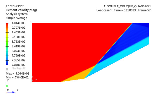
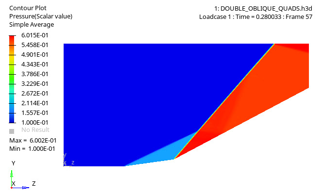
It is interesting to take a look at pressure element velocity and density once steady-state is reached.


Figure 4. Contour for Elemental Velocity


Figure 5. Contour for Elemental Pressure
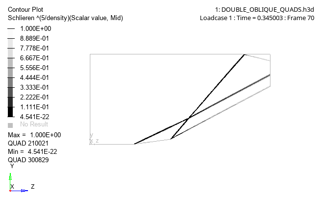
The Schlieren contour highlights the shock fronts. To improve the view of the shock waves from the Schlieren output, advanced math was used in HyperView. The /H3D/ELEM/SCHLIEREN output was raised to the 5th power and the legend changed to greyscale with black at the minimum and white for the maximum value.


Figure 6. Schlieren Output to the Power of (5/density)
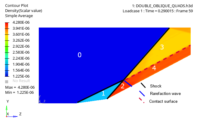
The shock front shown in Figure 7 divides the flow into four states as each shock front slows down and recompresses.


Figure 7. Shock Fronts and Density Map Showing the different States

Fluid particles close to the wall go through two shock fronts, while those away from the wall see only one. However, it is stronger, so flow quantities in State 3 differ from State 2. State 2 and State 4 are separated by a verification wave, with allows for a pressure equilibrium between States 3 and 4. All other quantities are otherwise discontinuous between State 3 and State 4, as the two are separated by a contact wave.

Results obtained from the simulation can be compared to the values obtained analytically.

Analytical Analysis

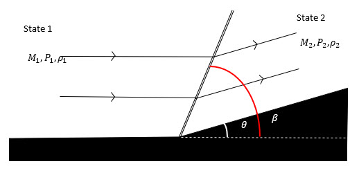
The shocks are created by the two wedges. These two obstacles slow down and recompress the flow as it changes direction and becomes parallel to the wedge. With supersonic flows, this process happens through an oblique shock wave, a stationary discontinuity which separates a pre-shock state (State 1), where the fluid is in this problem moving along the z-axis, from a post-shock state (State 2), with increased pressure and mass density, but a lower velocity, as well as a new direction, parallel to the wedge.


Figure 8. Deflection of Supersonic Flow through an Oblique Shock

The theoretical values of thermodynamic quantities in every state can be determined analytically.

First, determine the angle of the shock β , from the flow Mach number M 1 MathType@MTEF@5@5@+= feaagKart1ev2aqatCvAUfeBSjuyZL2yd9gzLbvyNv2CaerbuLwBLn hiov2DGi1BTfMBaeXatLxBI9gBaerbd9wDYLwzYbItLDharqqtubsr 4rNCHbGeaGqiVu0Je9sqqrpepC0xbbL8F4rqGqFfpeea0xe9vq=Jb9 vqpeea0xd9q8qiYRWxGi6xij=hbba9q8aq0=yq=He9q8qiLsFr0=vr 0=vr0db8meaabaqaciGacaGaaeqabaWaaeaaeaaakeaacaWGnbWaaS baaSqaaiaaigdaaeqaaaaa@3921@ and the wedge angle θ , by solving:(7) 1 tan ( θ ) = ( γ + 1 2 M 1 2 M 1 2 sin ( β ) 2 1 1 ) tan ( β ) MathType@MTEF@5@5@+= feaagKart1ev2aqatCvAUfeBSjuyZL2yd9gzLbvyNv2CaerbuLwBLn hiov2DGi1BTfMBaeXatLxBI9gBaerbd9wDYLwzYbItLDharqqtubsr 4rNCHbGeaGqiVu0Je9sqqrpepC0xbbL8F4rqGqFfpeea0xe9vq=Jb9 vqpeea0xd9q8qiYRWxGi6xij=hbba9q8aq0=yq=He9q8qiLsFr0=vr 0=vr0db8meaabaqaciGacaGaaeqabaWaaeaaeaaakeaadaWcaaqaai aabgdaaeaaciGG0bGaaiyyaiaac6gadaqadaqaaiabeI7aXbGaayjk aiaawMcaaaaacqGH9aqpdaqadaqaamaalaaabaGaeq4SdCMaey4kaS IaaGymaaqaaiaaikdaaaWaaSaaaeaacaWGnbWaaSbaaSqaaiaaigda aeqaaOWaaWbaaSqabeaacaaIYaaaaaGcbaGaamytamaaBaaaleaaca aIXaaabeaakmaaCaaaleqabaGaaGOmaaaakiGacohacaGGPbGaaiOB amaabmaabaGaeqOSdigacaGLOaGaayzkaaWaaWbaaSqabeaacaaIYa aaaOGaeyOeI0IaaGymaaaacqGHsislcaaIXaaacaGLOaGaayzkaaGa ciiDaiaacggacaGGUbWaaeWaaeaacqaHYoGyaiaawIcacaGLPaaaaa a@5A97@
Rankine-Hugoniot Jump formulas for the oblique shock are then used to obtain the values in post-shock state:(8) P 2 P 1 = 2 γ M 1 2 sin ( β ) 2 γ + 1 γ + 1 MathType@MTEF@5@5@+= feaagKart1ev2aqatCvAUfeBSjuyZL2yd9gzLbvyNv2CaerbuLwBLn hiov2DGi1BTfMBaeXatLxBI9gBaerbd9wDYLwzYbItLDharqqtubsr 4rNCHbGeaGqiVu0Je9sqqrpepC0xbbL8F4rqGqFfpeea0xe9vq=Jb9 vqpeea0xd9q8qiYRWxGi6xij=hbba9q8aq0=yq=He9q8qiLsFr0=vr 0=vr0db8meaabaqaciGacaGaaeqabaWaaeaaeaaakeaadaWcaaqaai aadcfadaWgaaWcbaGaaGOmaaqabaaakeaacaWGqbWaaSbaaSqaaiaa igdaaeqaaaaakiabg2da9maalaaabaGaaeOmaiabeo7aNjaad2eada WgaaWcbaGaaGymaaqabaGcdaahaaWcbeqaaiaaikdaaaGcciGGZbGa aiyAaiaac6gadaqadaqaaiabek7aIbGaayjkaiaawMcaamaaCaaale qabaGaaGOmaaaakiabgkHiTiabeo7aNjabgUcaRiaaigdaaeaacqaH ZoWzcqGHRaWkcaaIXaaaaaaa@4F97@ (9) ρ 2 ρ 1 = ( γ + 1 ) M 1 2 sin ( β ) 2 2 + ( γ 1 ) M 1 2 sin ( β ) 2 MathType@MTEF@5@5@+= feaagKart1ev2aqatCvAUfeBSjuyZL2yd9gzLbvyNv2CaerbuLwBLn hiov2DGi1BTfMBaeXatLxBI9gBaerbd9wDYLwzYbItLDharqqtubsr 4rNCHbGeaGqiVu0Je9sqqrpepC0xbbL8F4rqGqFfpeea0xe9vq=Jb9 vqpeea0xd9q8qiYRWxGi6xij=hbba9q8aq0=yq=He9q8qiLsFr0=vr 0=vr0db8meaabaqaciGacaGaaeqabaWaaeaaeaaakeaadaWcaaqaai abeg8aYnaaBaaaleaacaaIYaaabeaaaOqaaiabeg8aYnaaBaaaleaa caaIXaaabeaaaaGccqGH9aqpdaWcaaqaamaabmaabaGaeq4SdCMaey 4kaSIaaGymaaGaayjkaiaawMcaaiaad2eadaWgaaWcbaGaaGymaaqa baGcdaahaaWcbeqaaiaaikdaaaGcciGGZbGaaiyAaiaac6gadaqada qaaiabek7aIbGaayjkaiaawMcaamaaCaaaleqabaGaaGOmaaaaaOqa aiaabkdacqGHRaWkdaqadaqaaiabeo7aNjabgkHiTiaaigdaaiaawI cacaGLPaaacaWGnbWaaSbaaSqaaiaaigdaaeqaaOWaaWbaaSqabeaa caaIYaaaaOGaci4CaiaacMgacaGGUbWaaeWaaeaacqaHYoGyaiaawI cacaGLPaaadaahaaWcbeqaaiaaikdaaaaaaaaa@5C79@

All the physical properties in State 1 and State 2 can thus be determined.

The determination of State 3 and State 4 is more complex. Stage 3 is separated from State 0 by a single oblique shock wave. However, this shock wave is not generated by a single wedge of known angle, but rather by the combination from the two other shocks.

The pressure in State 2 and 3 is not the same because the flow went through two successive oblique shock waves, instead of through one stronger shock front. A verification process will happen after State 2 until the pressure has decreased to its value in the adjacent State 3.

State 3 and 4 needs to be determined together. State 3 is obtained from a flow initially in state 0 that encounters an oblique shock (which angle β 3 MathType@MTEF@5@5@+= feaagKart1ev2aqatCvAUfeBSjuyZL2yd9gzLbvyNv2CaerbuLwBLn hiov2DGi1BTfMBaeXatLxBI9gBaerbd9wDYLwzYbItLDharqqtubsr 4rNCHbGeaGqiVu0Je9sqqrpepC0xbbL8F4rqGqFfpeea0xe9vq=Jb9 vqpeea0xd9q8qiYRWxGi6xij=hbba9q8aq0=yq=He9q8qiLsFr0=vr 0=vr0db8meaabaqaciGacaGaaeqabaWaaeaaeaaakeaacqaHYoGyda WgaaWcbaGaae4maaqabaaaaa@39EB@ in unknown) and shares the same pressure that State 4. The State 4 pressure is obtained after an isentropic verification from State 2, in which the Mach number of the flow changes from M 2 MathType@MTEF@5@5@+= feaagKart1ev2aqatCvAUfeBSjuyZL2yd9gzLbvyNv2CaerbuLwBLn hiov2DGi1BTfMBaeXatLxBI9gBaerbd9wDYLwzYbItLDharqqtubsr 4rNCHbGeaGqiVu0Je9sqqrpepC0xbbL8F4rqGqFfpeea0xe9vq=Jb9 vqpeea0xd9q8qiYRWxGi6xij=hbba9q8aq0=yq=He9q8qiLsFr0=vr 0=vr0db8meaabaqaciGacaGaaeqabaWaaeaaeaaakeaacaWGnbWaaS baaSqaaiaabkdaaeqaaaaa@391B@ to M 4 MathType@MTEF@5@5@+= feaagKart1ev2aqatCvAUfeBSjuyZL2yd9gzLbvyNv2CaerbuLwBLn hiov2DGi1BTfMBaeXatLxBI9gBaerbd9wDYLwzYbItLDharqqtubsr 4rNCHbGeaGqiVu0Je9sqqrpepC0xbbL8F4rqGqFfpeea0xe9vq=Jb9 vqpeea0xd9q8qiYRWxGi6xij=hbba9q8aq0=yq=He9q8qiLsFr0=vr 0=vr0db8meaabaqaciGacaGaaeqabaWaaeaaeaaakeaacaWGnbWaaS baaSqaaiaabkdaaeqaaaaa@391B@ .

The value of pressure in these two states is thus obtained by finding solutions of the following system (with P 4 MathType@MTEF@5@5@+= feaagKart1ev2aqatCvAUfeBSjuyZL2yd9gzLbvyNv2CaerbuLwBLn hiov2DGi1BTfMBaeXatLxBI9gBaerbd9wDYLwzYbItLDharqqtubsr 4rNCHbGeaGqiVu0Je9sqqrpepC0xbbL8F4rqGqFfpeea0xe9vq=Jb9 vqpeea0xd9q8qiYRWxGi6xij=hbba9q8aq0=yq=He9q8qiLsFr0=vr 0=vr0db8meaabaqaciGacaGaaeqabaWaaeaaeaaakeaacaWGqbWaaS baaSqaaiaabodaaeqaaaaa@391F@ = P 3 MathType@MTEF@5@5@+= feaagKart1ev2aqatCvAUfeBSjuyZL2yd9gzLbvyNv2CaerbuLwBLn hiov2DGi1BTfMBaeXatLxBI9gBaerbd9wDYLwzYbItLDharqqtubsr 4rNCHbGeaGqiVu0Je9sqqrpepC0xbbL8F4rqGqFfpeea0xe9vq=Jb9 vqpeea0xd9q8qiYRWxGi6xij=hbba9q8aq0=yq=He9q8qiLsFr0=vr 0=vr0db8meaabaqaciGacaGaaeqabaWaaeaaeaaakeaacaWGqbWaaS baaSqaaiaabodaaeqaaaaa@391F@ ), and the unknowns are β 3 MathType@MTEF@5@5@+= feaagKart1ev2aqatCvAUfeBSjuyZL2yd9gzLbvyNv2CaerbuLwBLn hiov2DGi1BTfMBaeXatLxBI9gBaerbd9wDYLwzYbItLDharqqtubsr 4rNCHbGeaGqiVu0Je9sqqrpepC0xbbL8F4rqGqFfpeea0xe9vq=Jb9 vqpeea0xd9q8qiYRWxGi6xij=hbba9q8aq0=yq=He9q8qiLsFr0=vr 0=vr0db8meaabaqaciGacaGaaeqabaWaaeaaeaaakeaacqaHYoGyda WgaaWcbaGaae4maaqabaaaaa@39EB@ and M 4 MathType@MTEF@5@5@+= feaagKart1ev2aqatCvAUfeBSjuyZL2yd9gzLbvyNv2CaerbuLwBLn hiov2DGi1BTfMBaeXatLxBI9gBaerbd9wDYLwzYbItLDharqqtubsr 4rNCHbGeaGqiVu0Je9sqqrpepC0xbbL8F4rqGqFfpeea0xe9vq=Jb9 vqpeea0xd9q8qiYRWxGi6xij=hbba9q8aq0=yq=He9q8qiLsFr0=vr 0=vr0db8meaabaqaciGacaGaaeqabaWaaeaaeaaakeaacaWGnbWaaS baaSqaaiaabkdaaeqaaaaa@391B@ .
P 3 P 0 = [ 2 γ γ +1 M 0 2 sin ( β 3 ) 2 γ 1 γ + 1 ] MathType@MTEF@5@5@+= feaagKart1ev2aqatCvAUfeBSjuyZL2yd9gzLbvyNv2CaerbuLwBLn hiov2DGi1BTfMBaeXatLxBI9gBaerbd9wDYLwzYbItLDharqqtubsr 4rNCHbGeaGqiVu0Je9sqqrpepC0xbbL8F4rqGqFfpeea0xe9vq=Jb9 vqpeea0xd9q8qiYRWxGi6xij=hbba9q8aq0=yq=He9q8qiLsFr0=vr 0=vr0db8meaabaqaciGacaGaaeqabaWaaeaaeaaakeaadaWcaaqaai aadcfadaWgaaWcbaGaae4maaqabaaakeaacaWGqbWaaSbaaSqaaiaa bcdaaeqaaaaakiabg2da9maadmaabaWaaSaaaeaacaqGYaGaeq4SdC gabaGaeq4SdCMaae4kaiaabgdaaaGaamytamaaBaaaleaacaqGWaaa beaakmaaCaaaleqabaGaaGOmaaaakiGacohacaGGPbGaaiOBamaabm aabaGaeqOSdi2aaSbaaSqaaiaaiodaaeqaaaGccaGLOaGaayzkaaWa aWbaaSqabeaacaaIYaaaaOGaeyOeI0YaaSaaaeaacqaHZoWzcqGHsi slcaaIXaaabaGaeq4SdCMaey4kaSIaaGymaaaaaiaawUfacaGLDbaa aaa@558A@
Oblique shock of angle β 3 MathType@MTEF@5@5@+= feaagKart1ev2aqatCvAUfeBSjuyZL2yd9gzLbvyNv2CaerbuLwBLn hiov2DGi1BTfMBaeXatLxBI9gBaerbd9wDYLwzYbItLDharqqtubsr 4rNCHbGeaGqiVu0Je9sqqrpepC0xbbL8F4rqGqFfpeea0xe9vq=Jb9 vqpeea0xd9q8qiYRWxGi6xij=hbba9q8aq0=yq=He9q8qiLsFr0=vr 0=vr0db8meaabaqaciGacaGaaeqabaWaaeaaeaaakeaacqaHYoGyda WgaaWcbaGaae4maaqabaaaaa@39EB@ between State 0 and State 3.


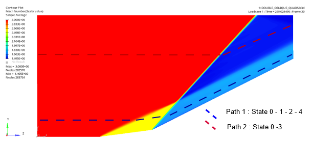
Figure 9. Mach Value Contour . w/o possible node paths going through every state of the flow
P 4 P 2 = ( 1+ γ -1 2 M 2 2 1+ γ -1 2 M 4 2 ) γ γ 1 MathType@MTEF@5@5@+= feaagKart1ev2aqatCvAUfeBSjuyZL2yd9gzLbvyNv2CaerbuLwBLn hiov2DGi1BTfMBaeXatLxBI9gBaerbd9wDYLwzYbItLDharqqtubsr 4rNCHbGeaGqiVu0Je9sqqrpepC0xbbL8F4rqGqFfpeea0xe9vq=Jb9 vqpeea0xd9q8qiYRWxGi6xij=hbba9q8aq0=yq=He9q8qiLsFr0=vr 0=vr0db8meaabaqaciGacaGaaeqabaWaaeaaeaaakeaadaWcaaqaai aadcfadaWgaaWcbaGaaeinaaqabaaakeaacaWGqbWaaSbaaSqaaiaa bkdaaeqaaaaakiabg2da9maabmaabaWaaSaaaeaacaqGXaGaae4kam aalaaabaGaeq4SdCMaaeylaiaabgdaaeaacaqGYaaaaiaad2eadaWg aaWcbaGaaeOmaaqabaGcdaahaaWcbeqaaiaaikdaaaaakeaacaqGXa Gaae4kamaalaaabaGaeq4SdCMaaeylaiaabgdaaeaacaqGYaaaaiaa d2eadaWgaaWcbaGaaeinaaqabaGcdaahaaWcbeqaaiaaikdaaaaaaa GccaGLOaGaayzkaaWaaWbaaSqabeaadaWcaaqaaiabeo7aNbqaaiab eo7aNjabgkHiTiaaigdaaaaaaaaa@5292@
Isentropic verification process from State 2 to State 4.

With β 3 MathType@MTEF@5@5@+= feaagKart1ev2aqatCvAUfeBSjuyZL2yd9gzLbvyNv2CaerbuLwBLn hiov2DGi1BTfMBaeXatLxBI9gBaerbd9wDYLwzYbItLDharqqtubsr 4rNCHbGeaGqiVu0Je9sqqrpepC0xbbL8F4rqGqFfpeea0xe9vq=Jb9 vqpeea0xd9q8qiYRWxGi6xij=hbba9q8aq0=yq=He9q8qiLsFr0=vr 0=vr0db8meaabaqaciGacaGaaeqabaWaaeaaeaaakeaacqaHYoGyda WgaaWcbaGaae4maaqabaaaaa@39EB@ and M 4 MathType@MTEF@5@5@+= feaagKart1ev2aqatCvAUfeBSjuyZL2yd9gzLbvyNv2CaerbuLwBLn hiov2DGi1BTfMBaeXatLxBI9gBaerbd9wDYLwzYbItLDharqqtubsr 4rNCHbGeaGqiVu0Je9sqqrpepC0xbbL8F4rqGqFfpeea0xe9vq=Jb9 vqpeea0xd9q8qiYRWxGi6xij=hbba9q8aq0=yq=He9q8qiLsFr0=vr 0=vr0db8meaabaqaciGacaGaaeqabaWaaeaaeaaakeaacaWGnbWaaS baaSqaaiaabkdaaeqaaaaa@391B@ determined, the other thermodynamics variables in State 4 are determined considering an isentropic rarefaction process from State 2 to State 4, and for State 3, by considering an oblique shock with an angle.

The solution of the double wedge problem using the shock polar. 1
Table 1. Analytical Results
  State 1 State 2 State 3 State 4
Shock angle [deg] 25.611 41.582 48.586 no shock
Mach number 2.603 1.722 1.537 1.746
Pressure [MPa] 0.180 0.595 0.574 0.574
Mass density [ g m m 3 ] MathType@MTEF@5@5@+= feaagKart1ev2aqatCvAUfeBSjuyZL2yd9gzLbvyNv2CaerbuLwBLn hiov2DGi1BTfMBaeXatLxBI9gBaerbd9wDYLwzYbItLDharqqtubsr 4rNCHbGeaGqiVu0Je9sqqrpepC0xbbL8F4rqGqFfpeea0xe9vq=Jb9 vqpeea0xd9q8qiYRWxGi6xij=hbba9q8aq0=yq=He9q8qiLsFr0=vr 0=vr0db8meaabaqaciGacaGaaeqabaWaaeaaeaaakeaadaWadaqaam aalaaabaGaai4zaaqaaiaac2gacaGGTbWaaWbaaSqabeaacaGGZaaa aaaaaOGaay5waiaaw2faaaaa@3D25@ 1.85E-06 4.15E-06 3.70E-06 4.04E-06

Numerical Results with Analytical Values Comparison

Numerical results for the thermodynamic variables can be read by drawing two node paths along two current lines, one close to the wall and going through State 1, 2 and 4, and the other further away from the wall, going from State 0 to State 3 (Figure 9).

To draw node paths, the elemental results visible on the animation have to be averaged at the nodes, using for example the averaging method simple.

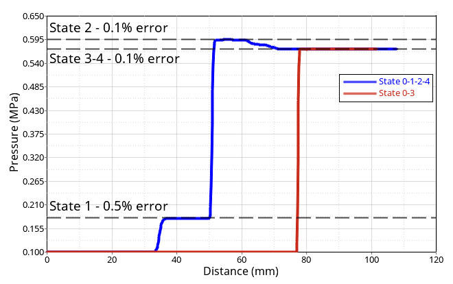
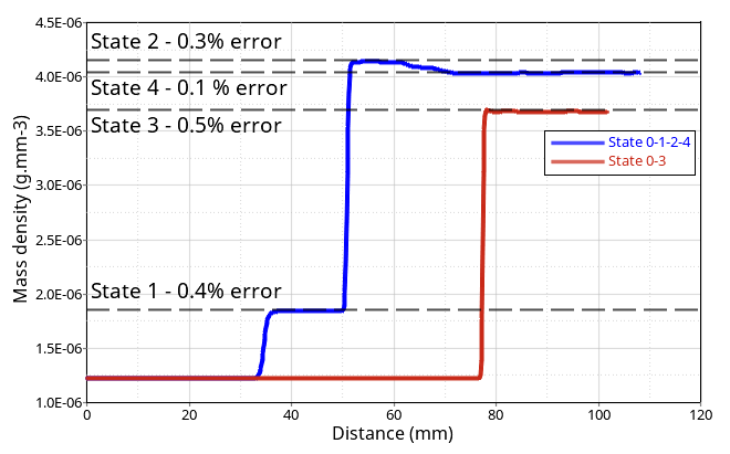
The spatial profile for pressure and mass density on these two nodes paths are visible on Figure 10 and Figure 11. Each flat on the curves corresponds to one the flow states described above. The value of the thermodynamic quantities obtained from the model can then be compared to those determined analytically.


Figure 10. Pressure Profile in Steady-State. with the value of the relative error to the analytical value


Figure 11. Mass Density Spatial Profile in Steady-State. with the value of the relative error to the analytical value
Analytical and numerical values for the flow Mach number in each state of the flow are compared.
Table 2. Analytical and Numerical Results for the Mach number
  Analytical Numerical Relative Error (%)
State 1 2.603 2.607 0.14
State 2 1.722 1.717 0.32
State 3 1.537 1.529 0.56
State 4 1.746 1.746 0.05

The relative error between numerical and analytical values for pressure, mass density and Mach number are for every state inferior to 1%.

Conclusion

Supersonic flow is modeled using a /MAT/LAW6 hydrodynamic fluid law, associated with an ideal gas equation of state (/EOS/IDEAL-GAS), within a multi-fluid material /MAT/LAW151 to use the finite volume solver.

As the flows encounters two wedges, three stationary shock waves and a contact wave are formed within the flow. The value of the flow physical parameters in each state can be determined analytically.

The analytical approach shows a good correlation between theoretical and numerical results.

The shocks and contact wave are rendered well on the simulation. The use of /MAT/MULTIFLUID allows for an accurate modeling of the dynamics of supersonic flows.

1 R. Courant, K.O. Friedrichs, Supersonic Flow and Shock Waves, Springer-Verlag, 1998