AFV-T: 3000 Transient Data
This tutorial shows you how to work with transient data. It also shows how to create streaklines to visualize transient flow patterns. An outline is presented for setting up rakes which can be used for subsequent work with other datasets.
Prior to running this tutorial, copy the expanded vortex_shedding directory from <AcuSolve installation directory>\model_files\tutorials\AcuFieldView\AFV_tutorial_inputs.zip to a working directory. See Tutorial Data for more information.
For Windows users, in order to take advantage of the restarts provided for this tutorial, you will need to make sure that the properties for your AcuFieldView shortcut on the Start menu do not include a Start in entry. To change that property, browse to the AcuFieldView shortcut on the Start menu, right-click, and select Properties. The Start in field can be found on the Shortcut tab in the AcuFieldView Properties dialog. Note that this step is only necessary because the restart files use relative paths.
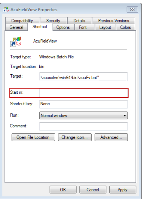
Figure 1.
Solve the Case with AcuConsole and AcuSolve
- Start AcuConsole.
- Open vortex_shedding.acs.
- Run AcuSolve to calculate a transient solution.
- Exit AcuConsole.
Convert the Dataset to FieldView Unstructured Format (FV-UNS)
- Open an AcuSolve Cmd Prompt or Linux terminal.
- Change the directory to the location of the solved problem, <your working dir>\vortex_shedding\.
- Execute AcuTrans with the following command line arguments: acuTrans -out -to fieldview -ts A -extout.
- Exit the command window or terminal when AcuTrans completes the conversion.
Start AcuFieldView and Read a Transient Dataset
-
Click and select white.
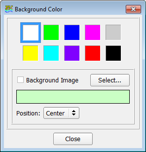
Figure 2. -
Click
 in the Transform Controls toolbar or to open the Defined Views panel.
-
Click Bound
 to visualize the cylinder using the Boundary Surface panel.
- Change Line Type to Thick and change the Geometric color to black.
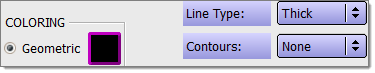
Figure 3. - Zoom into the cylinder (with Object set as World on the Viewer toolbar) with the right mouse button (M3).
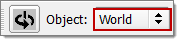
Figure 4. -
Click Coord
 to visualize the vortex shedding using the Coordinate Surface panel.
- Change the COLORING to Scalar and the DISPLAY TYPE from Mesh to Contours.
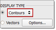
Figure 5. -
In the Colormap tab in the Coordinate Surface panel, change the Number of
Contours to 32 and the Colormap from Spectrum to
NASA-1.
You can also set the colormap on the Scalar Colormap Specification panel from the Edit menu.
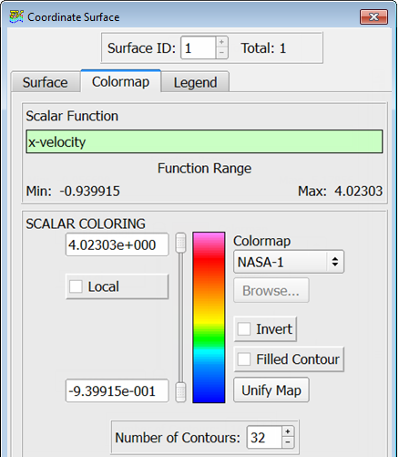
Figure 6. -
On the View menu turn off the Axis Markers and Perspective.
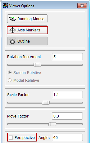
Figure 7.Note: The image on your screen may differ from what is shown based on the zoom level.
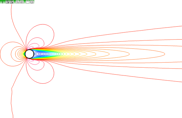
Figure 8.
Perform a Transient Sweep
-
Activate Sweep.The flow contours develop from a symmetric initial condition to the transient vortex shedding seen as the blue contours of the vortex "tail" sweeping up and down. Notice that the vertical extent of the "tail" is approximately that of the unit cylinder, and note that the center of the cylinder is the point [0,0,0]. This information will be used to create a "grid" in the following steps.
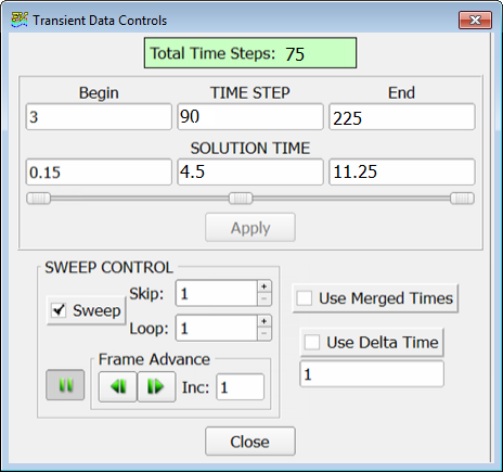
Figure 9. - Click Sweep to stop the animation.The following image is from time step 201.
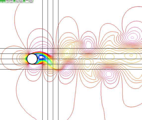
Figure 10.
Create Streamline Seeding Surfaces
-
Click the
 icon.
icon.
-
Change Max in the Threshold Function section to 0.25.
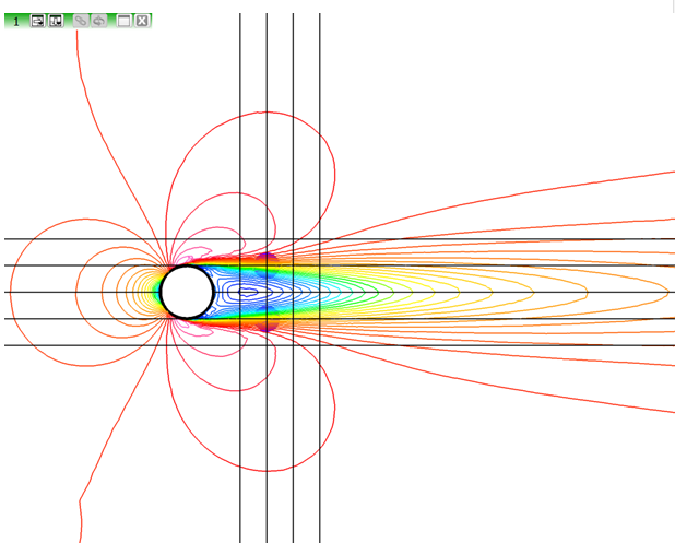
Figure 11.
Create Streamlines
-
Click Stream
 .
.
- Change the seeding Mode from Add (default) to Seed a Surface.
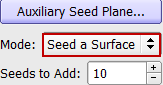
Figure 12. - Make the following changes to the Calculation Parameters at the bottom of the Streamlines panel (you may need to scroll down to see the bottom panel).
-
Increase the Step size from the default of 3 to 9.
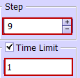
Figure 13.
-
Increase the Step size from the default of 3 to 9.
-
In the Streakline Parameters section, change the Release Interval to
1.
This will be used in streakline calculations later on.
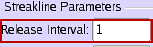
Figure 14. - Create a second rake and repeat the above steps as necessary for the other threshold coordinate surface.You may need to scroll up to see the top of the panel.
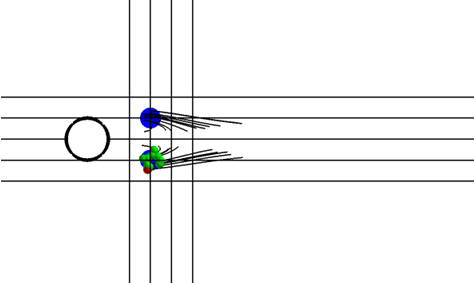
Figure 15.
Create Streaklines
-
Click Anno
 to open the
Annotation panel.
Tip: To see the icon on the toolbar, you might need to expand the toolbar with the
to open the
Annotation panel.
Tip: To see the icon on the toolbar, you might need to expand the toolbar with the icon.
icon. -
In the Annotation Create panel, enter in the
string:
Time Step: %%N1 Solution Time:
                                                  %%T1
and click OK.The special notation%%N1means show the time step of dataset #1 and%%T1means show the solution time of dataset #1.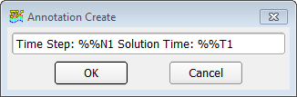
Figure 16. -
Move the title with the Shift+left mouse (M1) following the
hints on the Annotation panel.
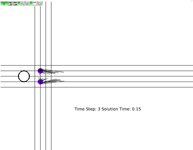
Figure 17. -
Click Frame Rate to open
the Minimum Time Between Frames panel and adjust
the Minimum Time Seconds to slow or speed up the
flipbook replay.
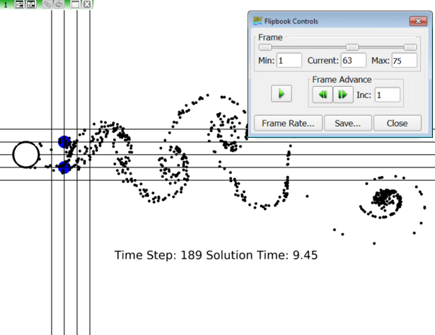
Figure 18.This image is from frame 63, which captured time step 189
Import Streaklines and Improve Your Animation
-
Click the Paths icon
 or .
or .
- Advance the TIME STEP to 225 and click Apply.This shows the positions of the particles at their furthest extent. When the TIME STEP slider is moved and applied, the positions of the particles change to match their locations at the selected time step.
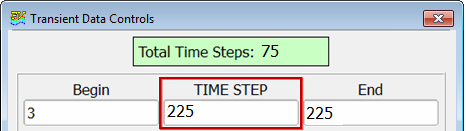
Figure 19. - Set Object to World on the Viewer toolbar.Resize the image in the modeling window so that more can be seen. Use zooming out (M3) and left translation (M1).
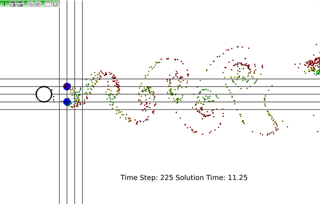
Figure 20. -
Save the flipbook as vortex_animation_1.avi when the creation is
complete.
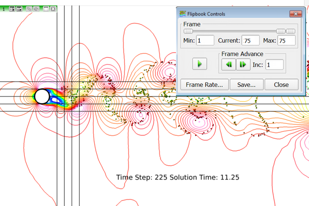
Figure 21.
Use Scripts
-
Click to read in the complete restart called
..\vortex_shedding\restart\vortex_shedding.dat.
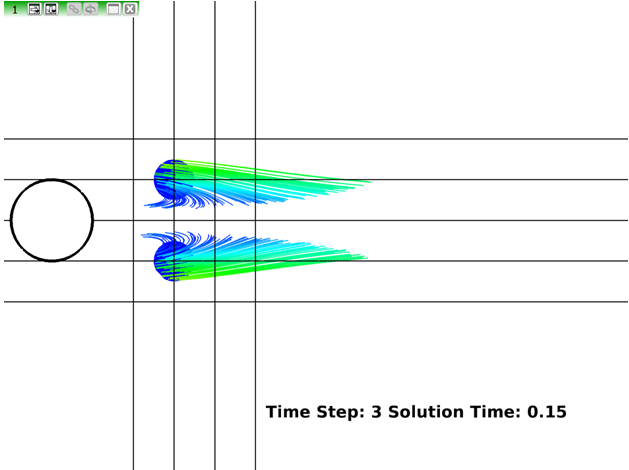
Figure 22. -
Click to read in the complete restart called
..\vortex_shedding\display_streakline.dat.
This restart imports the streaklines as particle paths, removes the coordinate lines, draws the cylinder using smooth shading, changes the view to better display the vortex shedding, sets the scalar function to use VecZ(curl(velocity)) for coordinate surface 1, relocates the surface plane to .05, and turns on presentation rendering for better looking particles.
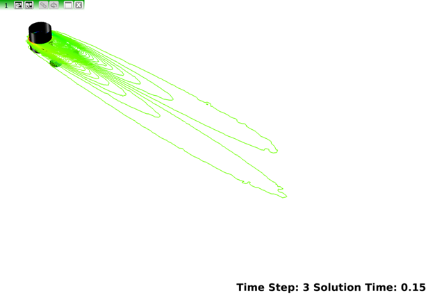
Figure 23.Note: You may need to resize your AcuFieldView window or move the model to get the view shown above. -
On the Colormap tab, change the scalar min/max values to
-10 and 40, respectively. The
Number of Contours should be 32. Alternately, these changes can be made using
the Scalar Colormap Specification panel.
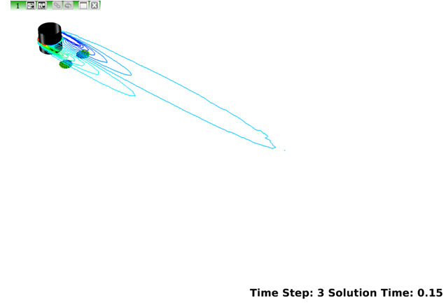
Figure 24. -
When the script completes, exit AcuFieldView (if
desired) and play the two flipbook animations, simple_streak and
final_streak.
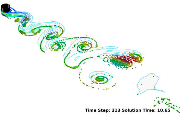
Figure 25. This image shows final_streak.avi at time step 213