ACU-T: 6010 Flow Through Porous Medium
Prerequisites
This tutorial provides the instructions for setting up, solving and viewing results for simulation of flow through a porous medium. Prior to starting this tutorial, you should have already run through the introductory HyperWorks tutorial, ACU-T: 1000 HyperWorks UI Introduction, and have a basic understanding of AcuSolve, HyperView, and HyperMesh. To run this simulation, you will need access to a licensed version of HyperMesh and AcuSolve.
Prior to running through this tutorial, copy HyperMesh_tutorial_inputs.zip from <Altair_installation_directory>\hwcfdsolvers\acusolve\win64\model_files\tutorials\AcuSolve to a local directory. Extract ACU-T6010_PorousMedia.hm from HyperMesh_tutorial_inputs.zip.
Since the HyperMesh database (.hm file) contains meshed geometry, this tutorial does not include steps related to geometry import and mesh generation.
Problem Description
The problem to be addressed in this tutorial is shown schematically in the figure below. It consists of a cylindrical channel with a porous medium in the flow section. As the flow passes through this section, a pressure drop is observed. In this simulation, an inlet velocity will be assigned to the flow and pressure drop across the porous medium will be calculated. The length of the porous section is 0.06 m and the fluid is an imaginary air-like fluid with a density of 1 kg/m3 and a molecular viscosity of 0.001 kg/m-s. The inlet velocity of the flow is 0.2 m/s.
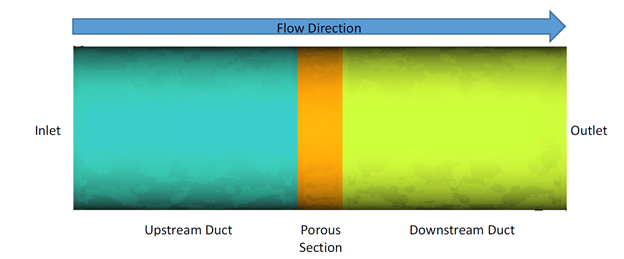
Figure 1.
Open the HyperMesh Model Database
-
Click the Open Model icon
 located on the standard toolbar.
The Open Model dialog opens.
located on the standard toolbar.
The Open Model dialog opens.
Set the General Simulation Parameters
In this step, you will set the simulation parameters that apply globally to the simulation.
-
In the Entity Editor, verify that the Analysis type is
set to Steady State and the Turbulence model is set to
Laminar.
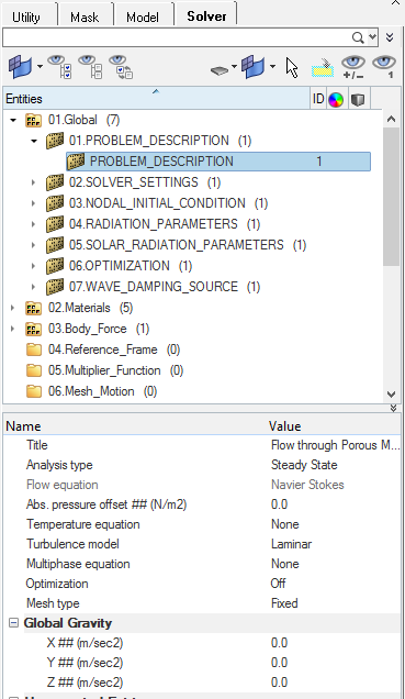
Figure 2.
Set Up Boundary Conditions and Material Model Parameters
In this step, you will start by modifying the material properties of Air and then create a material model for the porous medium. Then, you will assign the surface boundary conditions and material properties for all the fluid volumes.
Create the Material Model
-
In the Entity Editor, change the Density to
1 kg/m3 and the Viscosity to
0.001 kg/m-sec.
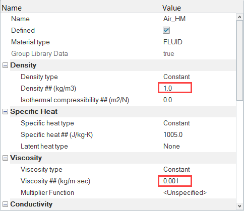
Figure 3. -
Set the Forchheimer coefficient to 8.33.
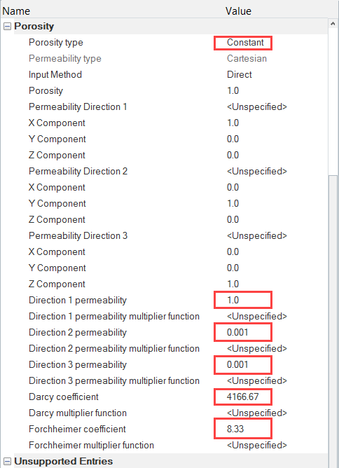
Figure 4.
Assign Boundary Conditions and Material Properties
-
Click Inlet. In the Entity Editor,
- Change the Type to INFLOW.
- Set the Inflow velocity type to Cartesian.
- Set the X velocity to 0.2 m/sec
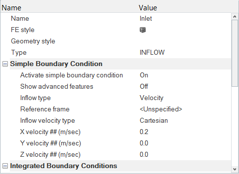
Figure 5. -
Click Outlet. In the Entity Editor, change the Type to OUTFLOW.
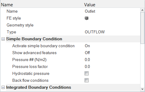
Figure 6. -
Click Walls. In the Entity Editor, verify that the Type is set to WALL.
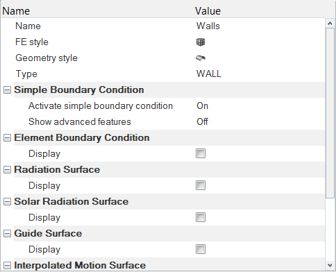
Figure 7.All the internal surfaces, such as the inlet and outlet of the porous section and the external walls of pipe surface, can be grouped into one single surface set. Auto_Wall, which is an advanced feature in AcuSolve, re-groups these elements into internal and external surfaces for each volume and writes the surface output accordingly. This process is done internally, thereby reducing the number of steps in the workflow.
-
Click Fluid_Upstream. In the Entity Editor,
- Change the Type to FLUID.
- Select Air_HM as the Material.
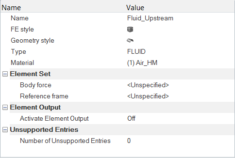
Figure 8. -
Click Fluid_Porous. In the Entity Editor,
- Change the Type to FLUID.
- Select Porous as the Material.
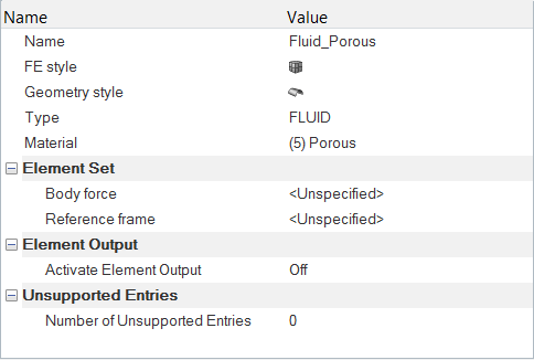
Figure 9. -
Click Fluid_Downstream. In the Entity Editor,
- Change the Type to FLUID.
- Select Air_Hm as the Material.
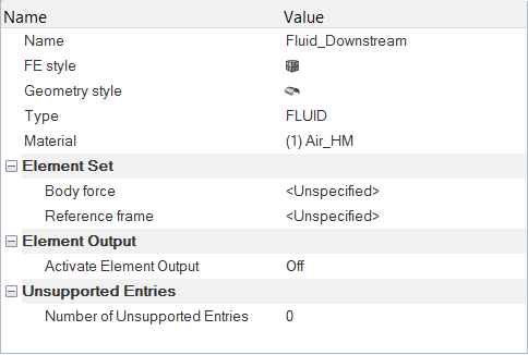
Figure 10.
Compute the Solution
In this step, you will launch AcuSolve directly from HyperMesh and compute the solution.
-
Click
 on the ACU toolbar.
The Solver job Launcher dialog opens.
on the ACU toolbar.
The Solver job Launcher dialog opens. -
Leave the remaining options as
default and click Launch to start the solution
process.
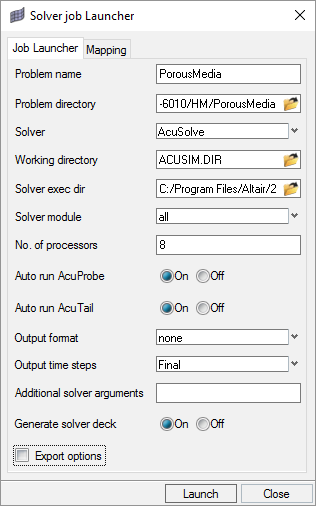
Figure 11.
Post-Process the Results
As the solution progresses, AcuProbe is launched automatically. AcuProbe can be used to monitor different variables over solution time. In this step, you will plot the residual ratio values and then compute the pressure drop across the porous section.
-
Right-click on Final and select Plot
All.
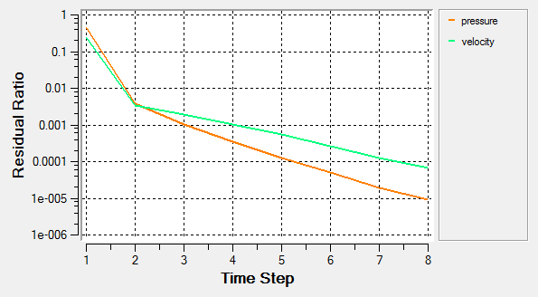
Figure 12. -
Click the User Function icon
 from the toolbar.
The User Function dialog opens.
from the toolbar.
The User Function dialog opens. -
Right-click on pressure and select Copy
name. Paste the value in the Function window after P_In =.
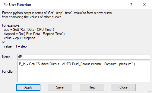
Figure 13. -
On the next line, type value = P_In - P_Out.
Note: The word “value” is case sensitive and should always be in lower case. If you use a capital letter, an error window appears.
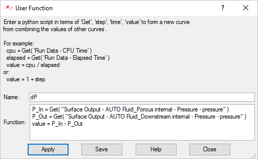
Figure 14. -
Click Apply to display the plot.
Note: You might need to click
 on the toolbar in order to
properly display the plot.
on the toolbar in order to
properly display the plot.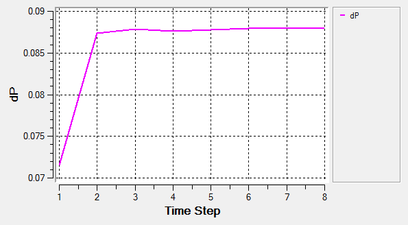
Figure 15.
Summary
In this tutorial, you learned how to set up and solve a problem with porous medium. You started by importing the HyperMesh database and then creating a material model for the porous section. Then, you assigned the boundary conditions and material properties and solved by launching AcuSolve directly from HyperMesh. Finally, you created a pressure drop plot using the user function tool in AcuProbe and calculated the drop in pressure between the inlet and outlet surfaces of the porous section.