ACU-T: 6000 Static Mixer Simulation - AcuTrace
This tutorial provides the instructions for setting up, solving and viewing results for a simulation of a static mixer in combination with the post-processing module AcuTrace. In this simulation, AcuSolve is used to compute the species mixing within a simple mixer and AcuTrace is used to compute the particle motion of finite mass particles within the mixer. This tutorial is designed to introduce you to concepts necessary to visualize streamlines and produce particle path with AcuTrace.
- Generation of finite mass particle paths with AcuTrace.
- Conversion of the nodal output data with AcuTranstrace for reading into AcuFieldView.
- Post-processing the nodal output with AcuFieldView to visualize streamlines and particle path.
Prerequisites
You should have already run through the introductory tutorial, ACU-T: 2000 Turbulent Flow in a Mixing Elbow. It is assumed that you have some familiarity with AcuConsole, AcuSolve, and AcuFieldView. You will also need access to a licensed version of AcuSolve.
Prior to running through this tutorial, copy AcuConsole_tutorial_inputs.zip from <Altair_installation_directory>\hwcfdsolvers\acusolve\win64\model_files\tutorials\AcuSolve to a local directory. Extract StaticMixer.acs from AcuConsole_tutorial_inputs.zip.
Analyze the Problem
An important step in any CFD simulation is to examine the engineering problem and determine the important parameters that need to be provided to AcuSolve. Parameters can be based on geometrical elements (such as inlets, outlets, or walls) and on flow conditions (such as fluid properties, velocity, or whether the flow should be modeled as turbulent or as laminar).
The problem to be addressed in this tutorial is shown schematically in Figure 1. It consists of a mixing tube that contains several swept walls to instigate mixing within the tube. The inlet face is split into two regions, one containing 100 percent of species_1 and the other containing zero.

Figure 1. Schematic of the static mixer
The boundary condition at the inlet is defined to produce a fully developed inlet profile with velocity of 1.0 m/s. One portion of the inlet is defined to contain 100 percent of species_1, while the other inlet is defined to contain 0.0 percent of species_1.
The fluid in this problem is an epoxy resin, which has a density of 1264.0 kg/m3 and a viscosity of 1.49 kg/m-sec.
In addition to setting appropriate conditions for the simulation, it is important to utilize a mesh that will be sufficiently refined to provide good results. In this application, the flow will accelerate as it passes over the fin walls. This leads to the higher gradients that need finer resolution. Proper boundary layer parameters need to be set to keep the y+ near the wall surface to a reasonable level. Although a slightly refined mesh is used in this area, it should be noted that a proper mesh refinement study is necessary in order to determine the required mesh controls to obtain a grid independent solution. The mesh controls used in this tutorial are very coarse and are only intended to illustrate the process of setting up the model and to retain a reasonable run time. A significantly higher mesh density is needed to achieve a grid converged solution.
Define the Simulation Parameters
Start AcuConsole and Create the Simulation Database
In the next steps you will start AcuConsole, and open the database for storage of the simulation settings. In this tutorial, you will begin by loading the existing database, preparing the particle trace settings and running the model. Next you run AcuTrace to generate the particle paths within the flow field and convert the data for reading into AcuConsole. Finally, you will visualize some characteristics of the results using AcuConsole.
- Start AcuConsole from the Windows Start menu by clicking .
- Click the File menu, then click Open to open the Chose a file dialog.
- Browse to the directory where StaticMixer.acs is stored.
- Select StaticMixer.acs and then click Open to open the database.
Set General Simulation Parameters
In next steps you will review parameters that apply globally to the simulation. To make this simple, the basic settings applicable for any simulation can be filtered using the BAS filter in the Data Tree Manager. This filter enables display of only a small subset of the available items in the Data Tree and makes navigation of the entries easier.
The general parameters that you will set for this tutorial are for turbulent flow, steady analysis, and mesh type as fixed.
-
Click BAS in the Data Tree Manager to switch to basic view in the Data Tree.
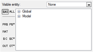
Figure 2. -
Double-click the Global
Data Tree item to expand it.
Tip: You can also expand a tree item by clicking
 next to the item name.
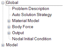
Figure 3. -
Set the Mesh type to Fixed.
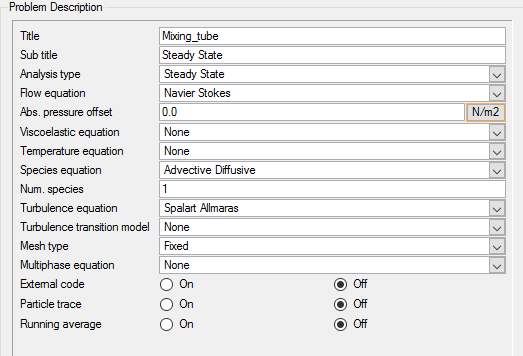
Figure 4.
Set Solution Strategy Parameters
Set Material Model Parameters
-
Double-click Material Model
in the Data Tree to expand it.
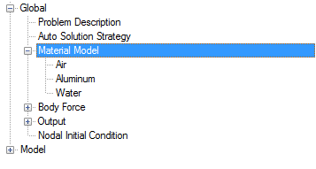
Figure 5. -
Save the database to create a backup
of your settings. This can be achieved with any of the following
methods.
- Click the File menu, then click Save.
- Click
 on
the toolbar.
on
the toolbar. - Click Ctrl+S.
Note: Changes made in AcuConsole are saved into the database file (.acs) as they are made. A save operation copies the database to a backup file, which can be used to reload the database from that saved state in the event that you do not want to commit future changes.
Prepare Output Data Stream
In order to utilize the finite mass particle trace functionality for particles that have non-constant density, you are required to store additional variables during the simulation. This is done by using the Derived Quantity Output mechanism.
- In the Data Tree, double-click Output to expand it.
- Double-click Nodal Output.
- Change the Time step frequency to 1000.
- Set the Time frequency to 0.
- In the Data Tree, double-click Derived Quantity Output to open the Derived Quantity Output detail panel.
- Change the Time step frequency to 1000.
- Set the Time frequency to 0.
Compute the Solution and Review the Results
Run AcuSolve
In the next steps you will launch AcuSolve to compute the solution for this case.
-
Click
 on the toolbar to open the
Launch AcuSolve dialog.
on the toolbar to open the
Launch AcuSolve dialog.
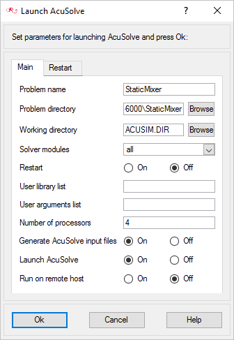
Figure 6.Note: For this case, the default values will be used. AcuSolve will run using four processors, and AcuConsole will generate AcuSolve input files and will launch AcuSolve. AcuSolve will calculate the steady state solution for this problem. -
Click Ok to start the
solution process.
While computing the solution, an AcuTail window opens. Solution progress is reported in this window. A summary of the solution process indicates that the run has been completed.
The information provided in the summary is based on the number of processors used by AcuSolve. If you use a different number of processors than indicated in this tutorial, the summary for your run may be slightly different than the summary shown.
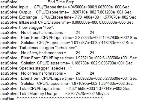
Figure 7.
Monitor the Solution with AcuProbe
AcuProbe can be used to monitor residuals.
-
Open AcuProbe by clicking
 on the toolbar.
-
Right-click on Final and select Plot
All.
The Solution ratio measures how much the solution is changing from one step to the next.Note: You might need to click
 on the toolbar in order to
properly display the plot.
on the toolbar in order to
properly display the plot.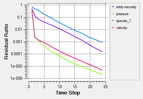
Figure 8.
Prepare Particle Trace Attribute for AcuTrace
Now that the steady-state simulation is complete, you can use the finite mass particle tracer to simulate micro-particles of SiO2, which are often used to add strength to the epoxy.
Define Particle Trace Parameters for Static Analysis
In the next steps you will define the particle trace data.
-
In the Data Tree, expand Particle
Trace to show only items related to particle tracing.
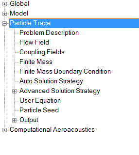
Figure 9.
Define Finite Mass Boundary Conditions
In the next steps you will set the finite mass boundary conditions.
-
Enter 0.2 for both the Normal and Tangential coefficient
of restitution.
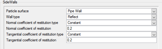
Figure 10. -
Enter 0.8 for both the Normal and Tangential coefficient
of restitution.
This will allow for less energy to be lost when the particle hits the wall and in turn will reflect off of the wall with a greater velocity.
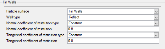
Figure 11.
Define Particle Seeds
In the next steps you will define the particle seeds that are moving into the flow regime.
-
For Constant radius, enter 0.0001.
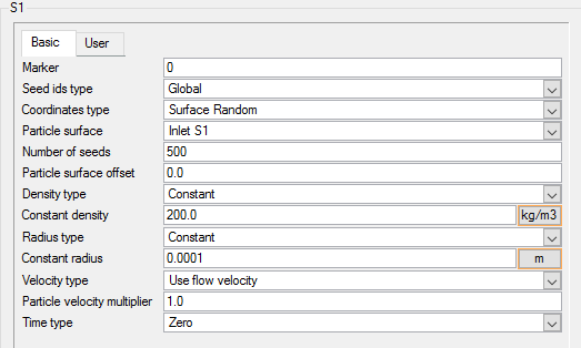
Figure 12. -
For Constant radius, enter 0.00015.
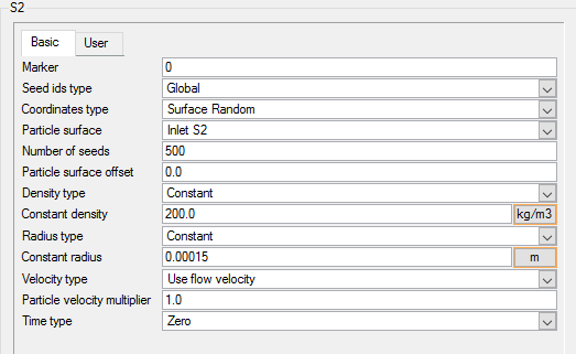
Figure 13.
Define the Output Parameters
In the next steps you will define the output parameters.
-
For Output frequency, enter 10.
This is equivalent to outputting the streamlines of the data at a frequency that relates the number of segments, or the approximate length of the particles. In order to reduce the amount of disc required in AcuTrace, it is recommended that the output frequency be larger than 1, more specifically, an order of magnitude larger.
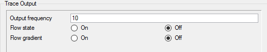
Figure 14.
Compute the Particle Paths and Review
Now that the steady-state simulation is complete, we can use the finite mass particle tracer to simulate micro-particles of SiO2 which are often used to add strength to the epoxy.
Run AcuTrace
In the next steps, you will launch AcuTrace to compute the solution for this case.
-
Click
 on the toolbar to open the
Launch AcuTrace dialog.
on the toolbar to open the
Launch AcuTrace dialog.
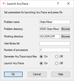
Figure 15.
Convert Results for AcuFieldView
Once the run is complete, you need to convert the results so that they can be read in AcuFieldView. To do this, run the AcuTransTrace utility. This tool can be used to convert data for Ensight, FieldView or AcuDisplay.
-
Enter the command:
acuTransTrace –to fieldview –fvopt streamline,steady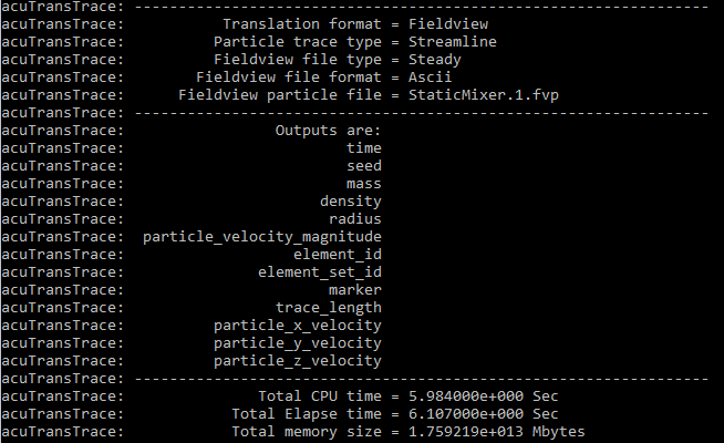
Figure 16.
Post-Process with AcuFieldView
- How to find the data readers in the File pull-down on the Main menu and open up the desired reader panel for data input.
- How to find the visualization panels either from the Side toolbar or the Visualization panel pull-downs on the Main menu to create and modify surfaces in AcuFieldView.
- How to move the data around the modeling window using mouse actions to translate, rotate and zoom in to the data.
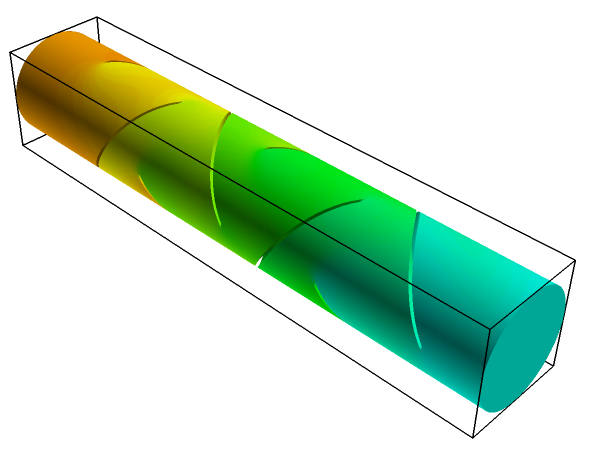
Figure 17.
Create a Boundary Surface and Coordinate Plane in Mixer
- In the Boundary Surfaces dialog, change the Coloring to Geometric.
- Select grey from the color tab.
- Uncheck the Show Mesh option to turn off the mesh display.
- From the Boundary Types list, select OSF: Fin Walls and click Ok.
- Orient the geometry to show that the flow moves from bottom to top of the screen.
- In the Boundary Surfaces dialog, click Create to create a new boundary surface.
- From the Boundary Types list, select OSF: Pipe Walls and click OK.
- Set the Display Type to Outlines and set Coloring to Geometric.
Set the Coordinate Surface Showing Velocity Magnitude on the Mid Coordinate Surface
-
Click
 to open
the Coordinate Surface dialog.
to open
the Coordinate Surface dialog.
-
Click the Legend tab, and activate the Show
Legend check box to display the velocity magnitude values on the
coordinate plane.
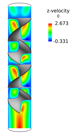
Figure 18.
Set the Boundary Surface and Particle Paths
-
Click the Paths icon
 to open the Particle
Paths dialog.
to open the Particle
Paths dialog.
-
Click the Legend tab and turn on the legend.
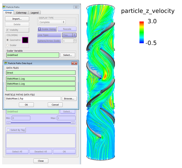
Figure 19.
Summary
In this tutorial, you successfully set up and solved for a steady simulation of a static mixer to visualize the particle path. You started the tutorial by opening a database in AcuConsole and setting up the simulation parameters to compute the species mixing within the mixer. You ran AcuTrace to generate the particle paths within the static mixer and converted the data using AcuTranstrace to visualize the particle paths in AcuFieldView.