ACU-T: 5301 Ship Hull Dynamics
This tutorial provides the instructions for setting up, solving, and viewing results of a flow around a freely floating ship hull. In this simulation, a wave hits the ship hull and displacement of the ship and the flow around the ship are simulated. This tutorial is designed to introduce you to a number of modeling concepts necessary to perform Free-Surface simulations.
- Use of Rigid Body type mesh motion
- Use of Free surface and Guide surface capabilities in conjunction of Rigid Body mesh motion.
- Analyze the problem
- Start AcuConsole and create a simulation database
- Set general problem parameters
- Use the pre-defined material model - Aluminum
- Create Rigid Body Mesh Motion
- Apply Mesh Motion to the Volume and Surface attributes
- Run AcuSolve
- Monitor the solution with AcuProbe
- Post-processing the nodal output with AcuFieldView
Prerequisites
In order to run this tutorial, you should have already run through the introductory tutorials, ACU-T: 2000 Turbulent Flow in a Mixing Elbow and ACU-T: 5300 Ship Hull Static, and be familiar with AcuConsole, AcuSolve, or AcuFieldView. In order to run this tutorial, you will need access to a licensed version of AcuSolve.
Prior to running through this tutorial, copy AcuConsole_tutorial_inputs.zip from <Altair_installation_directory>\hwcfdsolvers\acusolve\win64\model_files\tutorials\AcuSolve to a local directory. Extract Ship_hull_static.acs and wave_c from AcuConsole_tutorial_inputs.zip.
Analyze the Problem
The problem to be addressed in this tutorial is shown below. It is a mid-section of a Wigley Ship model. Wigley hulls have been widely used as test cases for evaluating hydrodynamic behavior of ships. The present tutorial demonstrates the simulation of gravity waves hitting a freely floating Wigley hull and evaluating the position of the hull with time. This tutorial is similar to the Ship Hull Static tutorial, except that the ship hull is freely floating as a rigid body compared to a static ship hull.

Figure 1. Schematic of a Ship Hull
Generation of Surface Gravity Waves

Figure 2. Gravity Waves
A linear solution of surface gravity wave propagation would result in the following equation for horizontal velocity of wave.
Where,
is the horizontal particle velocity of wave
is the speed of the wave
U is the velocity amplitude of disturbance
is wave number =
is the wave length of the wave
is the depth of the water
is the frequency of the wave =
is the time period of the wave
t is the time
In the present simulation, the following values are used for the variables of above equation:
U = 0.1256 m/s
= 1.0 sec
= 12.566 m-1
= 0.01 m/s
= 0.5 m
In the present tutorial, at the inlet you will generate the wave for 2 seconds and simulate the motion of the wave for 5 seconds. A UDF (wave.c) written in C language is used for this purpose. For the details of the functions used in the wave.c, refer to the AcuSolve User-Defined Functions Manual.
Two Dimensional Simulations in AcuSolve
AcuSolve does not support a CFD analysis on a 2D surface mesh. However, a 2D analysis can be simulated on a volume mesh by having a single element extrusion along the perpendicular direction of 2D surface of interest and then having identical boundary conditions of symmetry or slip on both sides of extrusion. This way you can ensure that the solution does not vary along the thickness (extrusion), which is essentially a 2D representation of the problem. The present tutorial uses this approach.
Modeling the Solid Ship Hull
For the present tutorial the following properties are assumed for the ship hull.
Material = Aluminum
Density = 2702 kg/m3
Body Center = (1.12971, 0.0, 0.0082984) m
Body Mass = 0.2038 kg
Body Weight = 0.2038 × 9.81 = 2.0 N
Components of Moments of Inertia (in kg m2):
= 0.00113969
= 0.0051392
= 0.004006
Rigid Body Dynamic Analysis
- Internal Forces/Moments: refers to the integrated fluid traction and moment
- External Forces/Moments: refers to the force and moment you specify
A local coordinate system is used to simplify the definition of the rigid body model and the solution of the equations of motion. The translational and rotational equations of motion are:
Where,
are the translational displacement, velocity and acceleration vectors, respectively as:
, ,
are the angular displacement, angular velocity and angular acceleration vectors, respectively as:
,,
is the mass of the body.
is the dyadic (moment of inertia) matrix of the body.
are the translational and rotational damping matrices, respectively.
are the translational and rotational stiffness matrices, respectively.
are the internal Forces and Moments from the fluid.
are the external Forces and Moments you specify.
Rigid Body Dynamics Analysis for a 2D Problem
- The displacements of the ship along its span (y-direction) is neglected.
- The axis of rotation for the ship is along the y-direction and the variables along other axis are neglected.
- Translational damping and stiffness matrices and their rotational equivalents are assumed to be zero.
- The only external force acting on the rigid body is the gravity force () along the z-axis.
- The external moments acting on the body is zero, because the only external force acting on the body is gravity which does not generate any moment.
For the present tutorial, a single element extrusion will be made along the y-axis. Based on the above assumptions, you arrive with:
, ,
, ,
The translational equations of the motion will be:
The rotational equations of the motion will be:
The only critical component of moment of inertia for the present tutorial is .
Define the Simulation Parameters
Start AcuConsole and Open the Simulation Database
In the next steps you will start AcuConsole and open a database that is set up for a Ship hull static simulation. You will then make appropriate changes to the database to take into account the dynamics of the ship motion.
-
Click the File menu, then click
Open to open the Choose a file
dialog.
Note: You can also open the Choose a file dialog by clicking
 on the
toolbar.
on the
toolbar.
Set General Simulation Parameters
In the next steps you will modify global attributes needed for the transient portion of the simulation.
-
Click BAS in the Data Tree Manager to switch to basic view in the Data Tree.
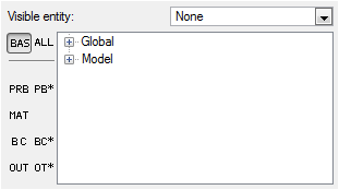
Figure 3. -
Double-click the Global
Data Tree item to expand it.
Tip: You can also expand a tree item by clicking
 next to the item name.
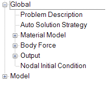
Figure 4. -
Name the Sub title as Ship hull dynamics.
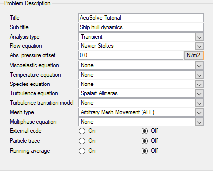
Figure 5.
Set Material Model Parameters
In the next steps you will verify that the pre-defined material properties of water and aluminum match the desired properties for this problem.
-
Double-click Material Model
in the Data Tree to expand it.
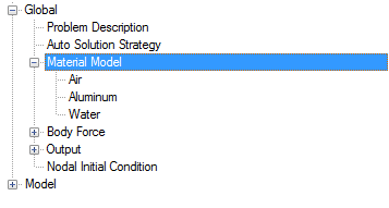
Figure 6. -
Save the database to create a backup
of your settings. This can be achieved with any of the following
methods.
- Click the File menu, then click Save.
- Click
 on
the toolbar.
on
the toolbar. - Click Ctrl+S.
Note: Changes made in AcuConsole are saved into the database file (.acs) as they are made. A save operation copies the database to a backup file, which can be used to reload the database from that saved state in the event that you do not want to commit future changes.
Set Mesh Motion Parameters
In the next steps you will define the mesh motion based on the rigid body dynamics of the ship hull.
-
For Mass, enter 0.2038 Kg.
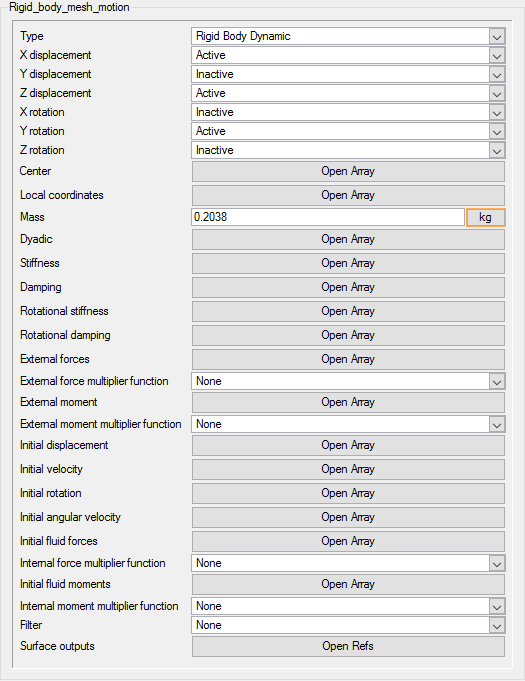
Figure 7. -
Enter the coordinates for the center of the ship hull, as shown below, and
click OK.
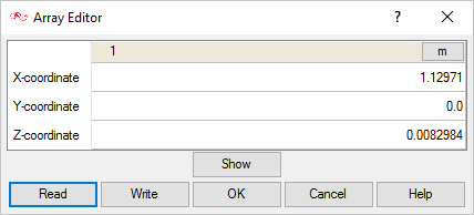
Figure 8.Local Coordinates: This parameter defines the direction of local xyz coordinate system, specified with respect to the global xyz coordinate system. -
Click Open Array adjacent to Local coordinates.
Since the local and global coordinates are same in this simulation, use the following defaults.
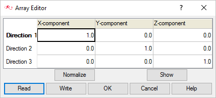
Figure 9. -
Click Open Array adjacent to Dyadic, and enter the
Moment of Inertia matrix, as shown below.
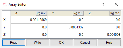
Figure 10.Though for the present 2D problem the only critical component of moment of inertia is Iyy as mentioned in the section Rigid Body Dynamics Analysis, AcuSolve would require the dyadic matrix to be positive definite because of the 3D volume mesh (refer to 2-Dimensional simulations in AcuSolve) and therefore, requires the input of Ixx, Izz.The parameters Stiffness, Damping, Rotational stiffness, and Rotational damping will be considered zero, because the ship is assumed to be freely floating on water.External forces: The force of gravity is the external force acting on the ship hull along the positive-z direction. -
Enter the Force vector as shown below and click
OK.
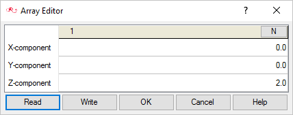
Figure 11.External Moment: The only external force on the ship hull is force of gravity. It does not produce any moment. Therefore, the External Moment will be zero in this simulation.The parameters Initial displacement, Initial velocity, Initial rotation, Initial angular velocity, Initial fluid forces, and Initial fluid moments will be considered zero, because of the stationary, equilibrium position of the ship considered at the start of the simulation.Surface outputs: This parameter lists the array of surfaces whose output of forces and moments will be enforced on the Rigid body (in this case, Ship hull). In this simulation, the forces from the fluid will be enforced on the ship hull through the surface “Hull_guide” of Fluid volume. -
Select Hull_guide and click OK.
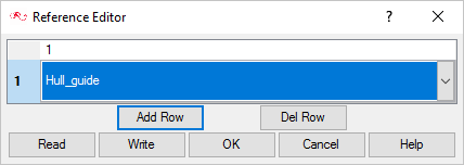
Figure 12.
Apply Volume Parameters
-
Change the Mesh motion to Rigid_body_mesh_motion.
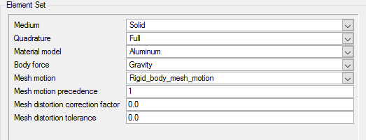
Figure 13.
Set the Mesh Motion to the Guide Surface
-
Change the Mesh motion to
Rigid_body_mesh_motion.
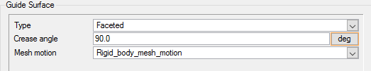
Figure 14.
Compile UDF for Windows
A UDF written in C language (wave.c) is provided with the tutorial. Now this C program should be compiled using the following steps.
Compile UDF for Linux
A UDF written in C language (wave.c) is provided with the tutorial. Now this C program should be compiled using the following steps.
Compute the Solution and Review the Results
Run AcuSolve
In the next steps you will launch AcuSolve to compute the solution for this case.
-
Click
 on the toolbar to open the
Launch AcuSolve dialog.
on the toolbar to open the
Launch AcuSolve dialog.
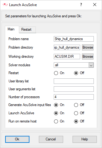
Figure 15.For this case, the default values will be used.
AcuSolve will run using four processors (if available, higher number of processors may be specified) and AcuConsole will generate AcuSolve input files and will launch AcuSolve. AcuSolve will calculate the transient solution for this problem.
-
Click Ok to start the
solution process.
While computing the solution, an AcuTail window opens. Solution progress is reported in this window. A summary of the solution process indicates that the run has been completed.
The information provided in the summary is based on the number of processors used by AcuSolve. If you use a different number of processors than indicated in this tutorial, the summary for your run may be slightly different than the summary shown.
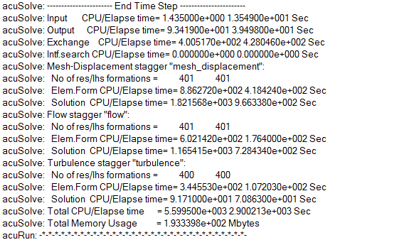
Figure 16.
Post-Process with AcuProbe
AcuProbe can be used to monitor various variables over solution time. In the present simulation it is worthwhile to monitor the forces on the ship hull.
-
Open AcuProbe by clicking
 on the toolbar.
-
Right-click on x_wall_shear_stress and click
Plot.
Note: You might need to click
 on the toolbar in order to
properly display the plot.
on the toolbar in order to
properly display the plot. -
Repeat the above steps for z_wall_shear_stress and click
Plot.
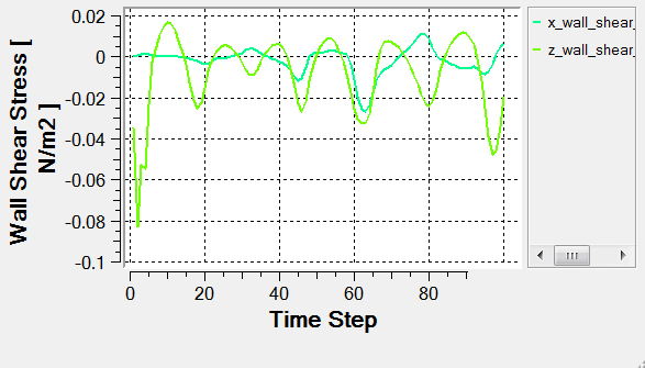
Figure 17.
View Results with AcuFieldView
Now that a solution has been calculated, you are ready to view the flow field using AcuFieldView. AcuFieldView is a third-party post-processing tool that is tightly integrated to AcuSolve. AcuFieldView can be started directly from AcuConsole, or it can be started from the Start menu, or from a command line. In this tutorial you will start AcuFieldView from AcuConsole after the solution is calculated by AcuSolve.
In the following steps you will start AcuFieldView, create an animation of the ship hull motion with the contours of z-mesh displacement.
Start AcuFieldView
-
Click
 on the
AcuConsole toolbar to open the
Launch AcuFieldView dialog.
on the
AcuConsole toolbar to open the
Launch AcuFieldView dialog.
Animate to View Displacement of the Ship
These steps are provided with the assumption that you are able to manipulate the view in AcuFieldView to have a white background, perspective turned off, outlines turned off, and the viewing direction set to +z. If you are unfamiliar with basic AcuFieldView operations, refer to Manipulate the Model View in AcuFieldView.
-
From the Colormap tab, turn on Local.
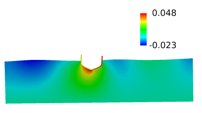
Figure 18. -
Click and move the slider all the way back to reflect the 1st time step
data on the boundary surfaces.
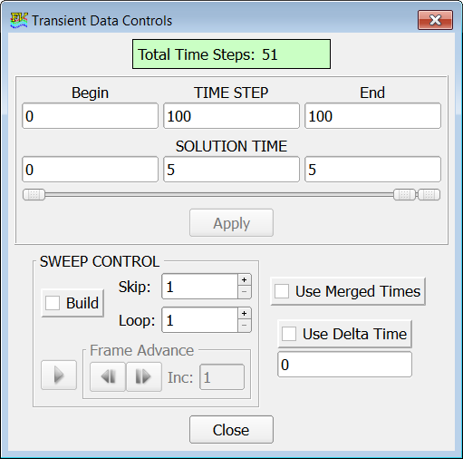
Figure 19.
Summary
In this tutorial, you worked through a basic workflow to set up a dynamic ship-hull simulation with surface gravity waves. You started with an .acs file from the Ship Hull Static tutorial and modified the set up to accommodate the rigid body motion of the ship hull. Once the case was set up, you generated a solution using AcuSolve. Results were post-processed in AcuFieldView to allow you to create animation of the Ship hull movement with time. New features introduced in this tutorial include: Rigid Body type mesh motion, use of Free surface and Guide surface capabilities in conjunction of Rigid Body mesh motion.