ACU-T: 5200 Rigid-Body Dynamics of a Check Valve
This tutorial provides the instructions for setting up, solving, and viewing results for a simulation of the opening of a pressure check valve. In this simulation, AcuSolve is used to compute the forces on the valve due to the time-varying inlet flow field and to compute the motion of the valve that results from these flow forces. This tutorial is designed to introduce you to a number of modeling concepts necessary to perform simulations of rigid-body dynamics.
Prerequisites
Prior to starting this tutorial, you should have already run through the introductory HyperWorks tutorial, ACU-T: 1000 HyperWorks UI Introduction, and have a basic understanding of HyperWorks CFD, AcuSolve, and HyperView. To run this simulation, you will need access to a licensed version of HyperWorks CFD and AcuSolve.
Prior to running through this tutorial, copy HyperWorksCFD_tutorial_inputs.zip from <Altair_installation_directory>\hwcfdsolvers\acusolve\win64\model_files\tutorials\AcuSolve to a local directory. Extract ACU-T5200_pressureCheckValve.x_t from HyperWorksCFD_tutorial_inputs.zip.
Problem Description
The problem to be addressed in this tutorial is shown schematically in Figure 1. It consists of a cylindrical pipe containing water that flows past a check valve with a shutter attached to a virtual spring (not included in the geometry). The inlet pressure varies over time and the movement of the shutter will be determined as a function of the balance of the fluid forces against the reactive force of the spring. The problem is rotationally periodic at 30° increments about the longitudinal axis, and it is assumed that the resulting flow is also rotationally periodic, allowing for modeling with the use of a wedge-shaped section. For this tutorial, a 30° section of the geometry is modeled, as shown in the figure. Modeling a portion of an rotationally periodic geometry leads to reduced computation time while still providing an accurate solution.

Figure 1. Schematic of Check Valve with Spring-Loaded Shutter
The pipe has an inlet diameter of 0.08 m, and is 0.3 m long. The check-valve assembly is 0.085 m downstream of the inlet. It consists of a plate 0.005 m thick with a centered orifice 0.044 m in diameter and a shutter with an initial position 0.005 m from the opening, simulating a nearly closed condition. The shutter plate is 0.05 m in diameter and 0.005 m thick. The shutter plate is attached to a stem 0.03 m long and 0.01 m in diameter. The mass of the shutter and stem is 0.2 kg and its motion is affected by a virtual spring with a stiffness of 2162 N/m. The motion of the valve shutter is limited by a stop mounted on a perforated plate downstream of the shutter.
Note that AcuSolve's internal rigid-body-dynamics solver is not able to simulate contact. Therefore, this problem is formulated to avoid contact between the valve and the stop.
- Scale up the fluid forces calculated by AcuSolve
by a factor of 12 to represent the full load on the device when the
displacement of the body is computed.
Using this approach, the full stiffness of the valve spring is used in the rigid-body solution, and the full mass of the valve is used.
- Scale down the mass of the valve and the stiffness of the spring to by a
factor of 12 to match the fraction of the valve geometry to be modeled.
Using this approach, the loading passed to the rigid-body solver is not scaled.
This second approach is used in this tutorial; the scaled mass of 0.0167 kg and the scaled stiffness of 180.1667 N/m will be used .
The fluid in this problem is water, which has a density (ρ) of 1000 kg/m3 and a molecular viscosity (μ) of 1 X 10⁻³ kg/m-sec.
At the start of the simulation the flow field is stationary. Flow is driven by the pressure at the inlet, which varies over time as a piecewise linear function shown in Figure 2. As the pressure at the inlet rises, the flow will accelerate as the valve opens. The turbulence viscosity ratio is assumed to be 10.
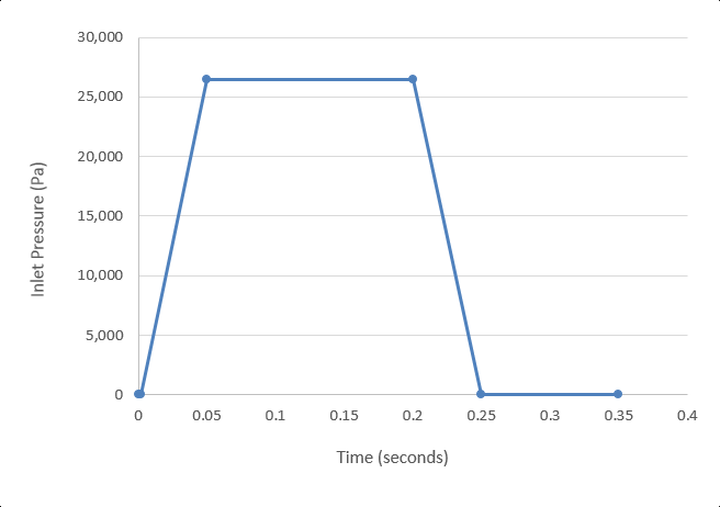
Figure 2. Transient Pressure at the Inlet
Prior simulations of this geometry indicate that the average velocity at the inlet reaches a maximum of 0.9 m/s. At this velocity, the Reynolds number for the flow is 72,000. When the Reynolds number is above 4,000, it is generally accepted that flow should be modeled as turbulent.
Note that the initial conditions of the flow are actually laminar, however, the increase in flow velocity and flow around the valve shutter is expected to cause a rapid transition to turbulent conditions. Therefore, the simulation will be set up to model transient, turbulent flow. When performing a transient analysis, convergence is achieved at every time step based on the defined stagger criteria. Mesh motion will be modeled using arbitrary mesh movement (arbitrary Lagrangian-Eulerian mesh motion).
For this case, the transient behavior of interest occurs in the time it takes for the pressure to ramp up and ramp back down, which is given by the transient pressure profile. To allow time for the spring to recover, additional time will be simulated. For this tutorial, 0.1 s is added after the pressure drops back to initial conditions, for a total duration of 0.35 s.
Another critical decision in a transient simulation is choosing the time increment. The time increment is the change in time during a given time step of the simulation. It is important to choose a time increment that is short enough to capture the changes in flow properties of interest, but does not require unnecessary computation time.
The change in inlet pressure from initial conditions to maximum occurs over 0.048 s. A time increment of 0.002 s would allow for excellent resolution of the transient changes, without requiring excessive computational time.
Start HyperWorks CFD and Create the HyperMesh Model Database
-
Create a new .hm database in
one of the following ways:
- From the menu bar, click .
- From the Home tools, Files tool group, click the Save As tool.
Figure 3.
Import and Validate the Geometry
Import the Geometry
-
In the Geometry Import Options dialog, leave all the
default options unchanged then click Import.
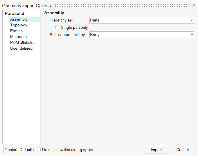
Figure 4.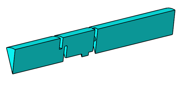
Figure 5.
Validate the Geometry
-
From the Geometry ribbon, click the Validate tool.

Figure 6.The Validate tool scans through the entire model, performs checks on the surfaces and solids, and flags any defects in the geometry, such as free edges, closed shells, intersections, duplicates, and slivers.The current model doesn’t have any of the issues mentioned above. Alternatively, if any issues are found, they are indicated by the number in the brackets adjacent to the tool name.
Observe that a blue check mark appears on the top-left corner of the Validate icon. This indicates that the tool found no issues with the geometry model.
Figure 7.
Set Up Flow
Set Up the Simulation Parameters and Solver Settings
-
From the Flow ribbon, click the Physics tool.

Figure 8.The Setup dialog opens. -
Under the Physics models setting:
- Set Time marching to Transient.
- Set the Time step size to 0.002 and the Final time to 0.35.
- Select Spalart-Allmaras as the Turbulence model.
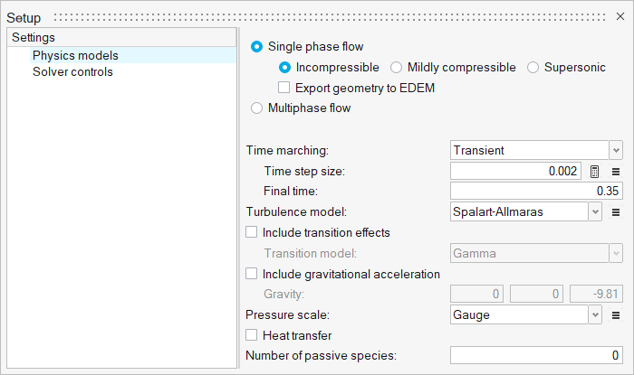
Figure 9. -
Click the Solver controls setting and set the Maximum
stagger iterations to 3.
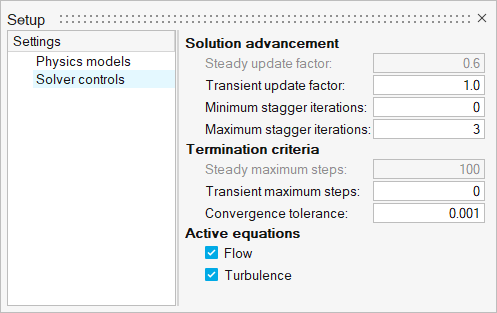 Figure 10.
Create a Multiplier Function for the Inlet Pressure
-
From the Flow ribbon, click the arrow next to the
Setup tool set, then select Multipliers.
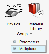
Figure 11. -
Click
 in the
Multiplier Library dialog.
in the
Multiplier Library dialog.
-
Click
 four
times to add four rows to the bottom of the table.
four
times to add four rows to the bottom of the table.
-
Enter the table values according to the image below.
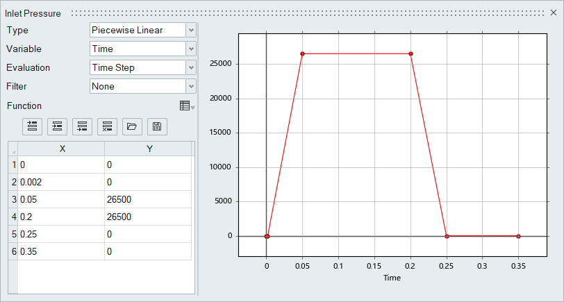
Figure 12.
Assign Material Properties
-
From the Flow ribbon, click the Material tool.

Figure 13. -
Click anywhere on the pipe geometry.
The entire geometry is highlighted.
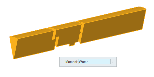
Figure 14. -
On the guide bar, click
 to execute
the command and exit the tool.
to execute
the command and exit the tool.
Define Flow Boundary Conditions
-
From the Flow ribbon, Pressure
tool group, click the Stagnation Pressure tool.

Figure 15. -
Click the Multiplier function drop-down and select the function
Inlet Pressure from the list.
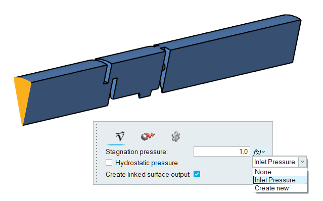
Figure 16. -
Click the Turbulence icon the microdialog, set the
Turbulence input type to Viscosity Ratio, and the enter a
value of 10 for the Turbulence viscosity ratio.
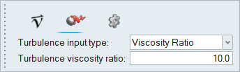
Figure 17. -
On the guide bar, click
 to execute the command and remain in the
tool.
to execute the command and remain in the
tool.
-
Click the Outlet tool.

Figure 18. -
Click the outlet surface shown in the figure below.
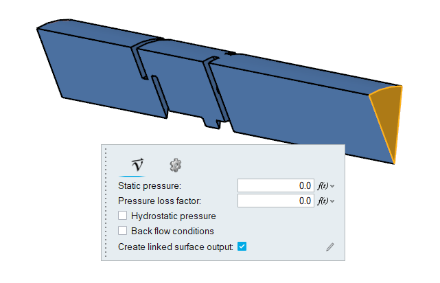
Figure 19. -
On the guide bar, click
to execute
the command and exit the tool.
-
Click the Symmetry tool.

Figure 20. -
Select the two surfaces shown in the figure below.
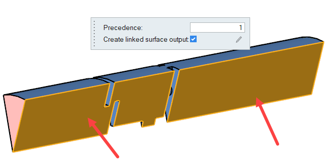
Figure 21. -
On the guide bar, click
to execute the command and remain in the
tool.
-
Rotate the model and select the other two symmetry faces.
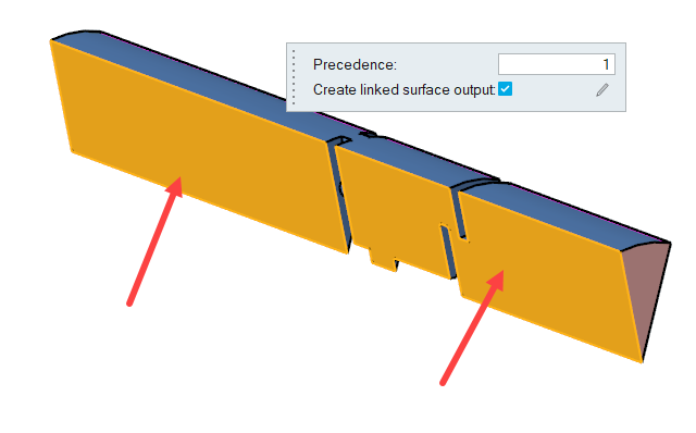
Figure 22. -
On the guide bar, click
to execute the command and remain in the
tool.
Set Up Motion
In this step, you will activate the mesh motion and define the rigid body motion for the valve wall. Then, you will define the mesh displacement boundary conditions for the symmetry surfaces.
Define the Mesh Motion Type
-
From the Motion ribbon, click the Settings tool.
Figure 23. -
In the Setup dialog, change the Mesh motion to
Arbitrary.
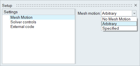
Figure 24.
Define Rigid Body Motion
-
From the Motion ribbon, click the Rigid Body tool.

Figure 25. -
For convenience, hide the Front_symmetry and Back_symmetry faces in the
modeling window by selecting the four surface and
then pressing H on the keyboard or by right-click and
selecting Hide from the context menu.
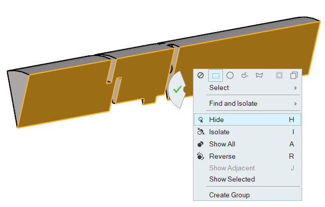
Figure 26. -
Select the valve wall surfaces, shown in the figure below, by using box
selection (hold and drag the left mouse button).
The number of surfaces selected should be 8, which will show on the guide bar.
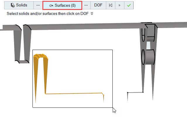
Figure 27. -
In the microdialog that appears, enter the following
values:
- Mass: 0.0167 kg
- Center: (0, 0, 0)
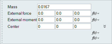
Figure 28. -
In the microdialog, enter a value of
180.1667 kg/sec2 for Kxx, the stiffness of
the spring.
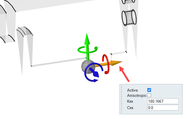
Figure 29. -
Click on the X-rotation arrow and de-activate it.
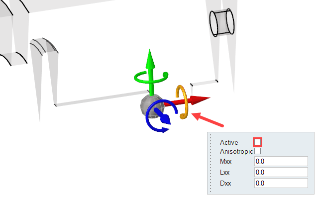
Figure 30. -
On the guide bar, click
to execute
the command and exit the tool.
Define the Mesh Displacement Boundary Conditions
-
From the Motion ribbon, click the Planar Slip tool.

Figure 31. -
In the Mesh Motion legend, rename Planar Slip to
Front_symmetry by double-clicking on the name.
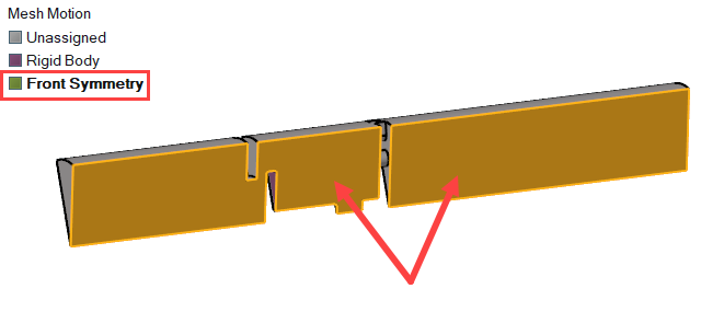
Figure 32. -
On the guide bar, click
to execute the command and remain in the
tool.
-
On the guide bar, click
to execute
the command and exit the tool.
Generate the Mesh
In this step, you will define the mesh controls and then generate the mesh.
Define the Zone Mesh Controls
-
From the Mesh ribbon, Zones
tool group, click the Cylinder
tool.

Figure 33. -
In the modeling window, hover the mouse around the
point shown in the figure below. When the preview cylinder zone is parallel to
the axis of the pipe, click on the model near the point shown below.
This point will be the center of the front face of the cylinder. In the next few steps you will edit the co-ordinates of this point manually.
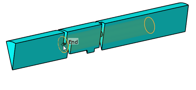
Figure 34. -
Move the mouse cursor away from the center and then click again.
A preview of the zone should be displayed on the screen along with the manipulator. The manipulator allows you to modify the location and orientation of the zone.
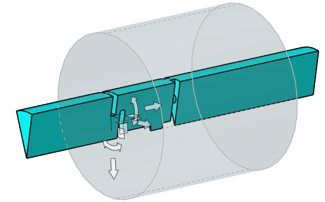
Figure 35. -
Click the center of the manipulator and enter the following coordinates for the
center (-0.06, 0.02, 0)
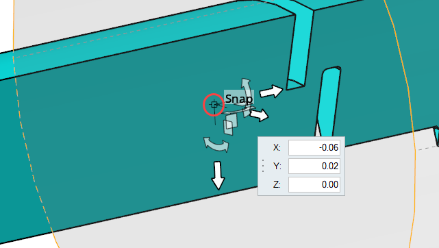
Figure 36. -
Double-click on the cylindrical surface of the zone and enter
0.022 m as the radius of the cylinder.
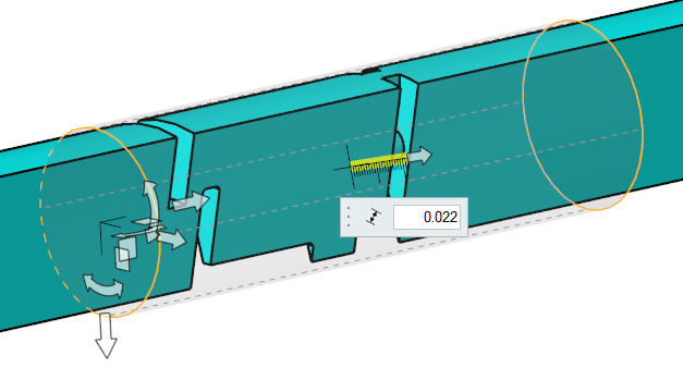
Figure 37. -
Double-click on the base of the cylinder and enter 0.1 m
as the height of the cylinder.
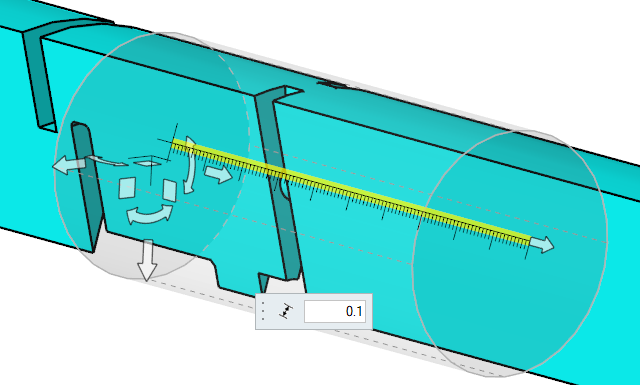
Figure 38. -
In the Refinement zones legend, rename the zone to Valve region mesh
refinement.
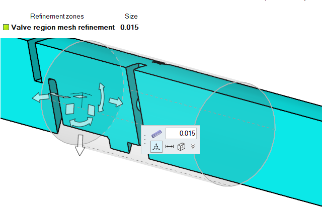
Figure 39.
Define the Boundary Layer Controls
-
From the Mesh ribbon, click the Boundary Layer tool.

Figure 40. -
Enter the following values in the dialog:
- First layer thickness: 0.00035
- Total number of layers: 3
- Growth method: Constant
- Initial growth rate: 1.2
- Termination policy: Truncate
- Activate Enable surface mesh modification.
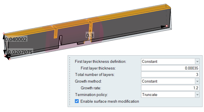
Figure 41. -
On the guide bar, click
to execute the command and remain in the
tool.
-
In the dialog that appears, enter the following values for the BL
specification:
- First layer thickness: 0.00015
- Total number of layers: 3
- Growth method: Constant
- Initial growth rate: 1.2
- Termination policy: Truncate
- Activate Enable surface mesh modification.
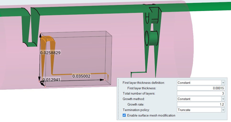
Figure 42. -
On the guide bar, click
to execute
the command and exit the tool.
-
Click the drop-down next to the Mesh Controls tool set and select Advanced.
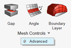
Figure 43. -
In the Advanced mesh settings dialog, change the Boundary
layer element type to Tetra then close the dialog.
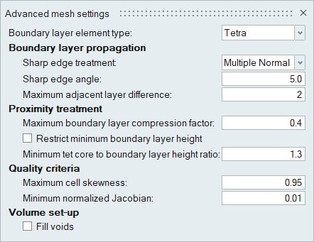
Figure 44.
Generate the Mesh
-
From the Mesh ribbon, click the Batch tool.

Figure 45. -
Click Mesh to generate the mesh.
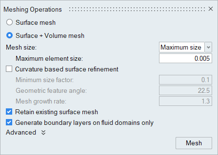
Figure 46.Once the meshing process has started, the Run Status dialog appears and the application moves to the Solution ribbon.
Compute the Solution
Define Nodal Outputs
-
From the Solution ribbon, click the Field tool.

Figure 47. -
In the Field Outputs dialog, set the Time step interval to
3 for the Solution variables.
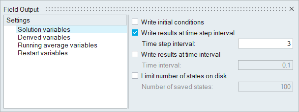
Figure 48.
Launch AcuSolve
-
From the Solution ribbon, click the Run tool.

Figure 49. -
Leave the remaining options as default and click
Run to launch AcuSolve.
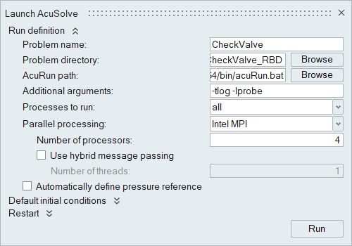
Figure 50.The Run Status dialog opens. Once the run is complete, the status is updated and you can close the dialog.
Monitor the Solution with AcuProbe
While AcuSolve is running, you can monitor flow characteristics such as inlet pressure, displacement of the valve, and velocity of the valve using AcuProbe.
-
Right-click on total_pressure and select
Plot.
Note: You might need to click
 on the toolbar in order to
properly display the plot.
on the toolbar in order to
properly display the plot.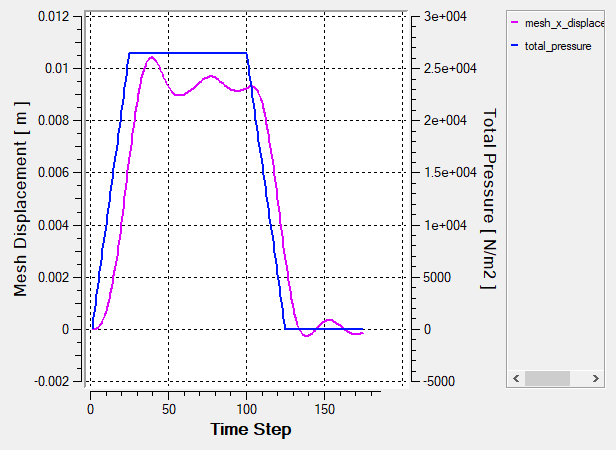
Figure 51.
Post-Process the Results with HyperView
In this step, you will create an animation of the valve motion as the water flows across the valve.
Open HyperView and Load the Model and Results
-
In the Load model and results panel, click
 next
to Load model.
next
to Load model.
Create an Animation of Velocity Magnitude
-
In Results Browser, expand the list of
Components and then click on the Isolate
Shown icon
 .
.
-
Click the Front_symmetry - Output component to turn off
the visibility of all the components except the front symmetry surface.
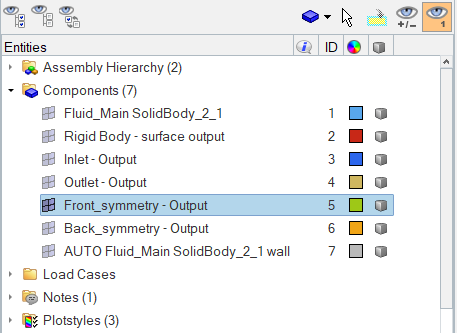
Figure 52. -
Orient the display to the xy-plane by clicking
 on the Standard Views toolbar.
-
Click
 on the Results toolbar to open the Contour panel.
-
Click the Components entity selector.
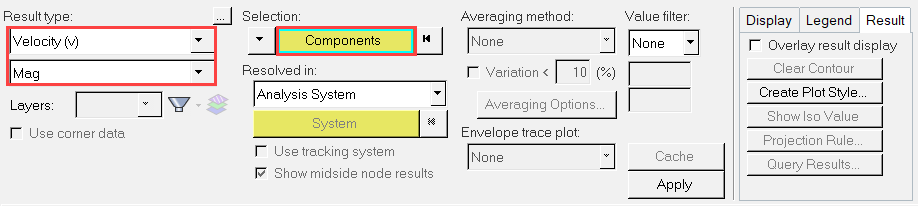
Figure 53. -
Click
 on the Animation toolbar to play the velocity magnitude
animation on the front symmetry plane.
on the Animation toolbar to play the velocity magnitude
animation on the front symmetry plane.
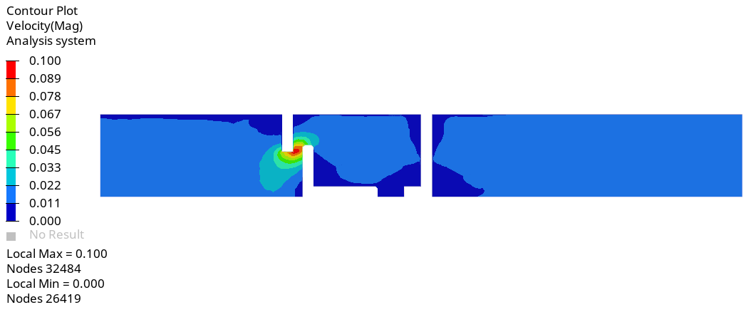
Figure 54. -
On the ImageCapture toolbar, click on the Capture Graphics Area
Video icon
 .
.
Display Pressure Contours and Velocity Vectors on a Section Cut
In the next step, you will create a section cut on the mid-z plane and then display the pressure contours and velocity vectors on that cross section.
-
In the Results Browser, turn off the display of all the
Components except the Fluid component (Fluid_Main_SolidBody_2_1).
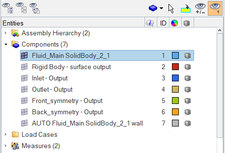
Figure 55. -
Click
on the Results toolbar to open the Contour panel.
-
In the panel area, under the
Result tab, activate the Overlay result
display check box (if not set already).
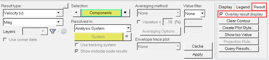
Figure 56. -
Click the Section cut icon
 on the HV-Display
toolbar.
on the HV-Display
toolbar.
-
Click the Vector icon
 on the Results toolbar to open the Vector panel.
-
Click the Selection drop-down and select
Sections from the list of options.
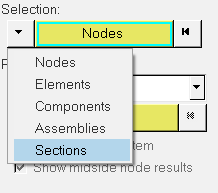
Figure 57. -
Set the Color by option to Direction and set the X+Y+Z
color to White.
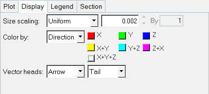
Figure 58. -
Go to the Section tab, activate the
Projected check box, then click
Apply.
The vector plot should look like the one shown in the figure below. The result at 0.156 sec is shown.
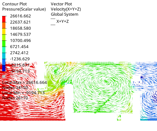
Figure 59.
Summary
In this tutorial, you learned how to set up and solve a CFD simulation involving rigid body mesh motion. You started by importing geometry, then defined the flow set up. Next, you defined the mesh motion set up and then generated the mesh. Once the solution was computed, you post-processed the results using AcuProbe and HyperView.