ACU-T: 5002 Brake Disc Cooling
in an Automotive Disc Brake System
This tutorial provides the instructions for setting up, solving and viewing results
for the simulation of a brake disc in a disc brake system, as well as understanding
the cooling mechanism of the disc. The model used for this tutorial consists of a
section of a brake disc on which a heat source is applied to simulate the braking
action. The heat source is the result of the friction between the brake disc that
rotates along with the wheel(s) and the brake pads, which are stationary with
respect to the wheel rotation. When the brake is applied, the pads are actuated by a
hydraulic mechanism and pressed against the disc. The frictional force between the
disc and the pads causes the deceleration of the disc, and hence the wheel. The most
common mechanism of the dissipation of the mechanical energy of the moving
automobile as it decelerates is through its conversion to heat energy due to
friction between the pad and the disc. The objective of this tutorial is to quantify
the temperature rise in a disc as a vehicle passes through a cycle of deceleration
and acceleration.
The basic steps in any CFD simulation are shown in ACU-T: 2000 Turbulent Flow in a Mixing Elbow. This tutorial does not introduce
any new concepts or feature capabilities of AcuSolve.
However, it does focus on demonstrating the capabilities of AcuSolve in successfully simulating a complex problem such as
a disc brake system and provides guidelines on how to setup a similar
simulation.
In this tutorial, you will:
Analyze the problem
Start AcuConsole and create a simulation
database
Set general problem parameters
Set solution strategy parameters
Import the geometry for the simulation
Create a volume group and apply volume parameters
Create surface groups and apply surface parameters
Set global and local meshing parameters
Generate the mesh
Run AcuSolve
Monitor the solution with AcuProbe
Post-process the solution with AcuFieldView
Prerequisites
You should have already run through the introductory tutorial, ACU-T: 2000 Turbulent Flow in a Mixing Elbow. It is assumed that you have some
familiarity with AcuConsole, AcuSolve, and AcuFieldView. You will
also need access to a licensed version of AcuSolve.
Prior to running through this tutorial, copy
AcuConsole_tutorial_inputs.zip from
<Altair_installation_directory>\hwcfdsolvers\acusolve\win64\model_files\tutorials\AcuSolve
to a local directory. Extract the files brake_disc_partial.x_t and heatSource.c and
the directory precursor_runfrom AcuConsole_tutorial_inputs.zip.
Analyze the Problem
An important step in any CFD simulation is to examine the engineering problem at hand and
determine the important parameters that need to be provided to AcuSolve. Parameters can be based on geometrical elements (such
as inlets, outlets, or walls) and on flow conditions (such as fluid properties,
velocity, or whether the flow should be modeled as turbulent or as laminar).
Figure 1 shows
the schematic and working mechanism of a typical disc brake system. The brake
pedal/lever is connected to the pushrod, which exerts force on the master cylinder
piston. Movement of the piston transfers the pressure applied on the piston through the
hydraulic lines to the brake pads, which are seated in the brake caliper assembly. The
pads are thus pushed towards the rotor, or the brake disc, exerting a friction force on
the rotating disc, causing it to decelerate till the brake lever is compressed by the
driver. The most common mechanism of the dissipation of the mechanical energy of the
moving automobile as it decelerates is through its conversion to heat energy due to
friction between the pad and the disc.
Figure 1. Model Used for the Simulation
The heat generated through the braking force can be very high under certain conditions,
and if not quickly dissipated to the ambient air, can cause significant temperature rise
in the disc. If the disc temperature rises beyond a certain limit, it can have
undesirable consequences on the braking performance, and in extreme cases can cause
brake failure as well. Some of these potential situations are listed below:
Downhill braking – when the vehicle cruising downhill for a long distance,
braking force is usually applied on the disc constantly to ensure the vehicle
speed is within a safe limit. Thus, the disc is placed under constant heating,
and the temperature of disc will keep rising until the heating is balanced by
cooling. The temperature reached at the ending state can be very high.
Repetitive braking is also a situation that often causes the disc temperature to
approach the safe limit. It is more commonly observed in racing where the
vehicle is always under deceleration or acceleration. Repetitive braking usually
consists of multiple brake-release cycles within a short time. In each cycle,
disc temperature rises during braking and then cools down in release time. At
the end of each cycle, the temperature may not be fully cooled down. As a
result, the temperature of disc gets higher and higher after each cycle and
eventually it may break the safe limit.
Emergency braking is also one of the reasons. Because the vehicle is stopped in
a very short time, the cooling effect is not significant enough to reduce the
temperature on disc. As a result, the temperature could be very high at the end
of the braking cycle
While modern disc brakes can safely operate up to a surface temperature of 1200 K, the
best operating range peeks out at about 900 K. Thus, this is the maximum temperature
most brake disc designs would strive to achieve, at least under normal braking.
Insufficient cooling of the brake system can result in thermal distortion, brake fading,
and brake fluid vaporization. Thermal distortion is due to excessive thermal expansion,
which in turn is due to high temperature; brake fading describes the friction force
between pad and disc, which under a fixed pressure reduces with increasing temperature.
High brake fluid temperature causes it to vaporize, which reduces the efficiency of the
hydraulic system. As a result, some brake pad stroke distance is wasted on compressing
gas.
A mechanical engineer is usually concerned about the following properties: brake fading
rate, thermal stress, thermal distortion, material strength limits, and brake fluid
temperature. In CFD simulations, all the concerns are related to the two outputs: disc
peak temperature and disc temperature distribution
Heat transfer Modes
There are three universal modes of heat transfer – conduction, convection and
radiation. All three modes are in play during a brake cooling cycle. The heat is
generated in the region where the brake pad and the brake disc are in contact, due
to friction between these two surfaces. A portion of the heat is conducted to the
pad and the remaining heat is absorbed by the disc. The heat is then dissipated in
the disc volume by conduction. The surface of the disc which is not in contact with
the pad dissipates the heat by convection and radiation.
All three heat transfer modes will be considered in this tutorial. However, modeling
of radiation heat transfer has been simplified by use of black body radiation theory
with no obstacles around the disc. For accurate radiation heat transfer, view
factors between the disc and the surrounding objects must be evaluated.
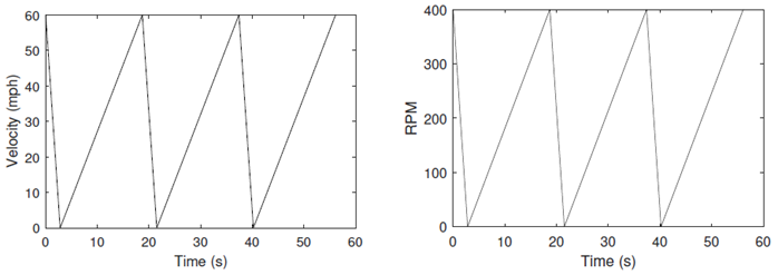
Simulation Scenario - Repetitive Braking
A repetitive braking scenario will be simulated in this tutorial. The initial speed
of the vehicle is assumed to be 60 mph, corresponding to a disc angular velocity of
400 rpm. The vehicle is brought to a stop through a linear deceleration process that
lasts 2.8 seconds. As soon as the vehicle speed hits zero, it linearly accelerates
again to a speed of 60 mph (400 rpm) for the next 15.9 seconds. The whole
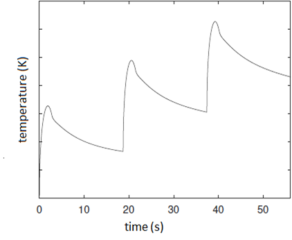
brake-release cycle thus lasts 18.7 seconds (figure 2). The first 2.8 seconds of
this cycle, that is the deceleration process, is the duration while the temperature
of the disc rises due to the heat generation caused by braking. In the following
15.9 seconds, the disc temperature falls as the heat is dissipated to the
surroundings. At the end of one such cycle, the brakes are applied again and the
disc temperature will rise once more (figure 3).
Figure 2. The Repetitive Brake-Release Scenario
Figure 3. Expected Temperature Rise in the Disc with the Progression of
Brake-Release Cycles
In this tutorial, two complete brake-release cycles will be evaluated.
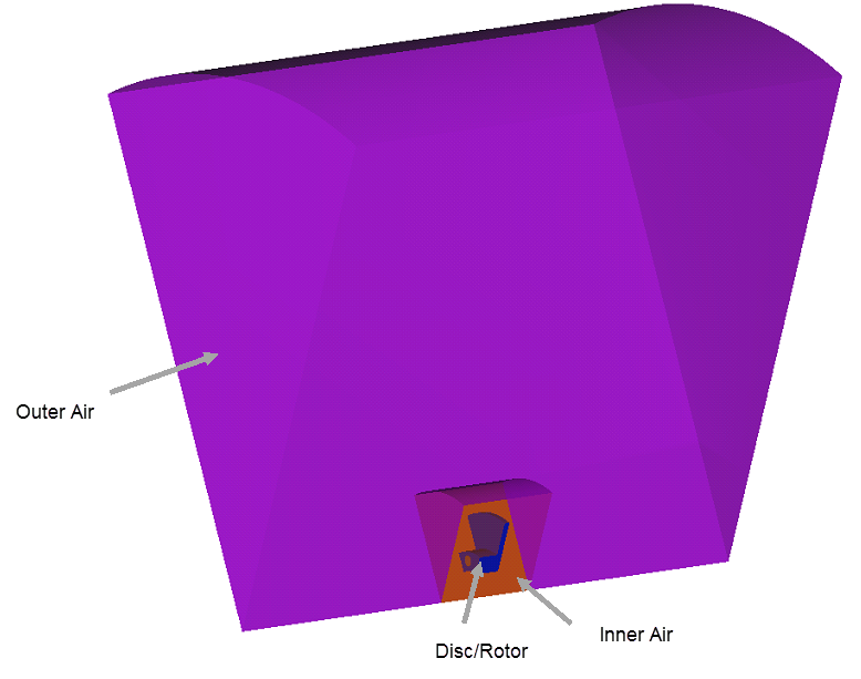
Disc Brake Geometry
For this tutorial, a section of the brake disc is being considered. Figure 4
shows the geometry that will be used for the simulation, which is a simplified
one-eighth (45 degree) section of the disc rotor. Note that the peripheral
components, like the pad, the caliper assembly, the wheel housing, etc., have not
been included.
Figure 4.
In the center of the domain is the disc. The inner air volume encloses the air volume
close to the disc. It represents the air volume inside the wheel, which rotates
along with the wheel. The outer air represents the ambient airflow. Thus, no moving
reference frame is required for the outer air. The disc has an outer radius of
0.15m, and the inner air radius is 0.2m. The ambient boundary is the outer surface
of the computational domain. It is a cylinder that is 1.1m tall with a radius of
1.0m. Note that in the current simulation, the vehicle body and other mechanical
parts are neglected. Essentially, this computational domain corresponds to an
idealized test rig in experiment. The air volume is just a simplification of the
outer environment of the brake disc.
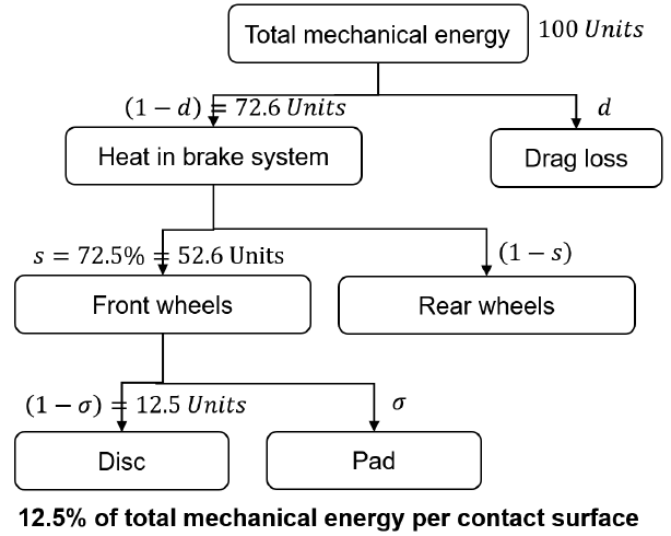
Heat Source Application
Figure 5
shows a schematic plot for estimating the energy flow through the braking system
when a brake is applied. Traversing through the plot, it can be seen that an
estimated 12.5% of the total mechanical energy of a moving vehicle is transferred to
each contact surface on the front wheel discs as the vehicle is brought to rest.
Figure 5. Energy Flow for Estimating Heat Flux on Front Wheel
Here, is the drag loss, which is around 27.4%. The
constant is the weight fraction on the front wheels,
estimated to be about 72.5%. The reference for these two constants can be found in
Martin (2004). The heat partition ratio σ = 0.05 is the heat transferred to the pad
surface. It can be estimated by equation 1 (Adamowicz and Grzes,
2011).
Here, is the conductivity, ρ is the density, and is the specific heat capacity. Subscript 1 refers to
the pad material and subscript 2 refers to the disc material.
If the braking process contains change in both potential energy and kinetic energy of
the vehicle, then the equation for calculating the heat flux becomes:
With the total mechanical energy,
In the current braking scenario, the vehicle is assumed to be moving on a plane road.
Thus, no change in potential energy is expected; only the kinetic energy of the
vehicle is transferred to heat.
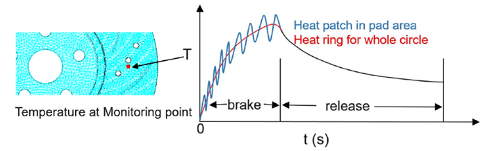
You have two options for determining the area of contact for the disc and pad surface.
In the first option, the actual area of contact between the disc and the pad is
considered. This is useful for a realistic simulation as it helps predict the peak
temperature that will be reached in the disc. If a monitoring point is put on the
disc surface, the temperature value for this monitoring point will rise and fall for
each revolution of the disc as it enters and exits the contact patch.
The second option is using an averaged heat source on the disc. In this case, the
heat flux generated within the contact patch is averaged over the circumferential
area swept by the disc-pad contact surface. This simplifies the simulation, but with
this option it is not possible to determine the peak temperature occurring in the
disc as the heat source itself is averaged.
Figure 6. Influence of Heat Patch on Temperature Variation at Monitoring
Point
The use of a heat source is also limited by the geometry used for the simulation. If
a partial disc geometry is used, you are restricted to an averaged heat source. This
tutorial will be setup using an averaged heat source applied on the disc. However,
for reference, following are the formulae used to calculate the area in equation …
for both the options.
For a realistic contact patch heat source,
For an averaged heat source,
Here, θ represents the sweep of brake pad on the disc. Averaged heat flux can be
computed based on realistic heat source as follows,
Based on the assumption that q is proportional to rpm and vehicle velocity, the heat
source from 0.0s to 2.8s can be given by,
For the provided geometry, the braking pad has a radius between ri = 0-11m and ro =
0-14m, and the pad sweep angle on disc surface is 60 degrees. This results in a
contact patch area of 0.003927 m2 on each side of the disc. The outer rim
radius of the disc is 0.15m, with a thickness of 0.016m at the outer rim of the
disc.
Note that in current simulations, the time function for the heat source is directly
defined in a UDF. The time function of the heat source is estimated from a
pre-defined velocity variation with time. To compute the heat source, you will need
the vehicle mass, velocity profile, and the help of some empirical coefficients
mentioned in Figure 5.
Simulation Options in AcuSolve
AcuSolve provides several options to represent the
physics of the problem when setting up the simulation. You will make use of some of
these options to represent the brake-release cycle and the relative motion between
the brake disc and the surrounding air.
One option to define the rotational motion of the disc is to use the sliding mesh
method. In this method, the actual physical motion of the brake disc in space is
simulated. However, it is not possible to use this method with the current geometry
since only a section of the disc is being modeled. As the disc rotates, it will
eventually move out of contact with the ambient air which is stationary. The correct
modeling option to define this is using a Moving Reference Frame (MRF) method. In
the MRF method, a reference frame is defined for the disc surface and the air
surrounding it. However, the disc itself is not rotated during the simulation.
The definition of the MRF which will be used for the disc surface and the air
surrounding it will have to take into account the changing rotational speed of the
disc as the vehicle decelerates and accelerates. This will be achieved using a
multiplier function which will be identical to the brake-release cycle curve shown
in Figure
2.
The heat source on the disc due to the braking is simulated using a user designed
function. Please refer the attached script heatSource.c. The
heat source is only applied when the brake is applied, and to the region where the
pad is in contact with the disc.
A precursor simulation is used to generate the initial conditions for the flow
quantities, i.e. pressure, velocity, and the eddy viscosity in the simulation
domain. It is assumed that the vehicle is cruising at a constant 60mph velocity
before applying brake. The temperature field before applying brake is considered
uniformly 300K, which doesn't need to be solved in precursor simulation. However,
the velocity field is not a steady state one because the air inside disc is rotating
along with the disc. Thus, only flow and turbulence equations are solved in this
precursor simulation. The results of this precursor simulation are provided in the
precursor_run directory. These results will be interpolated to
define the initial flow field for this simulation.
Define the Simulation Parameters
Start AcuConsole and Create the Simulation Database
In this tutorial, you will begin by creating a database, populating the
geometry-independent settings, loading the geometry, creating volume and surface
groups, setting group parameters, adding geometry components to groups, and
assigning mesh controls and boundary conditions to the groups. Next you will
generate a mesh and run AcuSolve to solve for the number
of time steps specified. Finally, you will visualize some characteristics of the
results using AcuProbe and AcuFieldView.
In the next steps you will start AcuConsole, and create
the database for storage of the simulation settings.
Start AcuConsole from the Windows Start menu by clicking Start > Altair <version> > AcuConsole.
Click the File menu, then click
New to open the New data
base dialog.
Note:You can also open the
New data base dialog by clicking on the toolbar.
Browse to the location that you would like to use as your working
directory.
This directory is where all files related to the simulation will
be stored. The AcuConsole database file
(.acs) is stored in
this directory. Once the mesh and solution are created, additional files and
directories will be created within this directory.
Create a new directory in this location. Name it
Brake_Cooling and open it.
Enter brake_cooling as the file name for the
database.
Note: In order for other applications to be able to read the
files written by AcuConsole, the database
path and name should not include spaces.
Click Save to create the database.
Set General Simulation Parameters
In next steps you will set parameters that apply globally to
the simulation. To make this simple, the basic settings applicable for any
simulation can be filtered using the BAS filter in the Data Tree Manager. This filter enables display of only a small subset
of the available items in the Data Tree and makes navigation
of the entries easier.
Click BAS in the Data Tree Manager to switch to basic view in the Data Tree.
Figure 7.
Double-click the GlobalData Tree item to expand it.
Tip: You can also expand a tree item
by clicking
next to the item name. Figure 8.
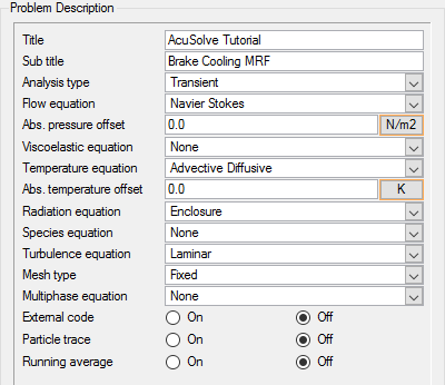
Double-click Problem
Description to open the Problem
Description detail panel.
Note: You may need to widen the detail panel from the default size by dragging
the right edge of the panel frame.
Enter AcuSolve Tutorial as the Title.
Enter Brake Cooling MRF as the Sub title.
Set the Analysis type to Transient.
Set the Temperature equation to Advective
Diffusive.
Set the Turbulence equation to Spalart Allmaras.
Set the Radiation equation to Enclosure.
Figure 9.
Set Solution Strategy Parameters
In the next steps you will set parameters that control the behavior of AcuSolve as it progresses during the solution.
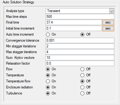
Double-click Auto Solution
Strategy to open the Auto Solution
Strategy detail panel.
Check that Analysis type is set to Transient.
Set the Max time steps to 500.
Set the Final time to 37.4 seconds.
Set the Initial time increment to 0.1 seconds.
Transient simulation will stop when either of the final time, or the Max time
steps is reached.
Set Min and Max stagger iterations to 2 and
4 respectively.
Check that the Flow, Temperature, Enclosure radiation, and Turbulence flags are
set to On, and the Temperature flow flag is set to Off.
Figure 10.
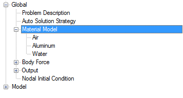
Set Material Model Parameters
AcuConsole has three pre-defined materials: Air,
Aluminum, and Water, with standard parameters defined. In the next steps you will verify
that the pre-defined material properties of air match the desired properties for this
problem. Subsequently, you will create a new custom material and assign relevant
material properties to it.
Double-click Material Model
in the Data Tree to expand it.
Figure 11.
Double-click Air in the
Data Tree to open the Air
detail panel.
The material type for air is Fluid. Fluid is
the default material type for any new material created in AcuConsole.
Click the Density tab. The density of air is 1.225 kg/m3
and the type is Constant.
Click the Viscosity tab. The viscosity of air is 1.781 x
10-5kg/m – sec and the type is Constant.
Similarly, check the Specific Heat and Conductivity tabs and make sure the
values are as follows:
Specific Heat: 1005.0 J/kg-K
Conductivity: 0.02521 W/m-K
Turbulent Prandtl number: 0.91
Save the database to create a backup
of your settings. This can be achieved with any of the following
methods.
Click the File menu, then click
Save.
Click on
the toolbar.
Click Ctrl+S.
Note: Changes made in AcuConsole are saved into
the database file (.acs) as they are made. A save operation copies the database to
a backup file, which can be used to reload the database from that saved
state in the event that you do not want to commit future changes.
Right-click on Material Model in the Data Tree and select New from the
context menu.
A new entry, Material Model 1, will be created in the Data Tree under the Material Model branch.
Rename the material model.
Right-click on Material Model 1.
Select Rename from the context menu.
Enter Disc Steel as the material name.
Press Enter on the keyboard.
Note: When an item in the Data Tree is renamed,
the change is not saved until you press the Enter. If you move the input focus away from the
item without entering it, your changes will be lost.
Double-click on Disc Steel in the Data Tree to open the material detail panel.
The material type is listed as Fluid. This is the default type for any new
material created in AcuConsole.
Click on the Material type drop-down selector and choose
Solid from the list that appears.
Set the material properties for Disc Steel as follows by navigating through the
respective tabs in the detail panel:
Density: 7200 kg/m3
Specific Heat: 537.0 J/kg-K
Conductivity: 45.0 W/m-K
Save the database to create a backup of your settings.
Import the Geometry and Define the Model
Import the Geometry
You will import the geometry in the next
part of this tutorial. You will need to know the location ofbrake_disc_partial.x_tin order to complete these steps. This file contains
information about the geometry in ParasolidASCII format.
Click File > Import.
Browse to the directory containing brake_disc_partial.x_t.
Change the file name filter to Parasolid File (*.x_t *.xmt *X_T
…).
Select brake_disc_partial.x_t and click
Open to open the Import Geometry
dialog.
Figure 12.
For this tutorial, the default values for the Import
Geometry dialog are used to load the geometry. If you have previously
used AcuConsole, be sure that any settings that you
might have altered are manually changed to match the default values shown in the
figure. With the default settings, volumes from the CAD model are added to a default
volume group. Surfaces from the CAD model are added to a default surface group. You
will work with groups later in this tutorial to create new groups, set flow
parameters, add geometric components, and set meshing parameters.
Click Ok to complete the geometry import.
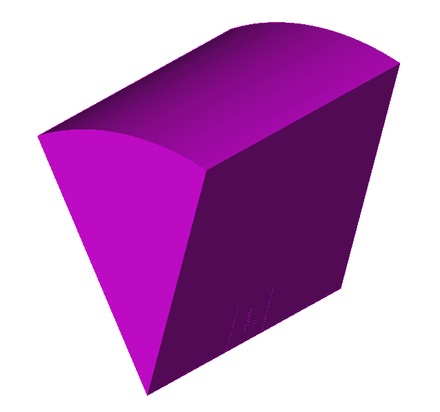
Rotate the visualization to view the entire model.
Figure 13.
The color of objects shown in the modeling window in this tutorial and those displayed on your screen may differ. The default color
scheme in AcuConsole is "random," in which colors are
randomly assigned to groups as they are created. In addition, this tutorial was
developed on Windows. If you are running this tutorial on a different operating system,
you may notice a slight difference between the images displayed on your screen and the
images shown in the tutorial.
Create a Multiplier Function for the Moving Reference Frame
As discussed in the introduction, a repetitive braking scenario is simulated in this
tutorial. The simulation starts at the instant the brake is applied. The initial
speed of the vehicle is 60 mph, corresponding to a disc rotor speed of 400 rpm. Over
the course of the simulation, the vehicle is decelerated to a speed of zero, then
accelerated back to 60 mph. The complete brake-release cycle is then repeated once
more. In AcuConsole, this behaviour will be represented
using a multiplier function. This multiplier function will later be assigned to the
definition of the moving reference frame, which will ultimately govern the motion of
the disc.
Click PB* in the Data Tree Manager to display all the available settings related to general problem setup in
the Data Tree.
Right-click on Multiplier Function and select
New from the context menu.
Rename the newly created multiplier function to
MRF_Multiplier.
Don't forget to press Enter after typing in the new
entity name.
Double-click on MRF_Multiplier to open the detail panel.
In the detail panel,
Change the Type to Piecewise Linear.
Set the Curve fit variable to Time.
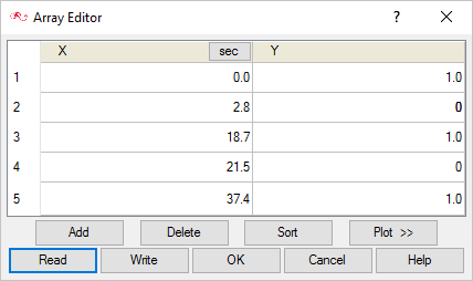
Click the Open Array button next to Curve fit
values.
In the Array Editor dialog, click the
Add button and create five rows.
Fill in the values as follows:
Figure 14.
Click OK to close the dialog.
Create Emissivity Models for Air and Disc
In this section, you will create and define the emissivity models for air and disc,
which will be used for the definition of radiation surfaces.
Click RAD in the Data Tree Manager
to filter all but the radiation relates settings in the Data Tree.
Right-click on Emissivity Model in the Data Tree and select New from the
context menu.
A new entry, Emissivity Model 1, will be created in the Data Tree under the Emissivity Model branch.
Repeat the previous step to create another entry, Emissivity Model 2.
Rename Emissivity Model 1.
Right-click on Emissivity Model 1.
Select Rename from the context menu.
Enter Disc Steel as the model name.
Press Enter on the keyboard.
In a similar manner, rename Emissivity Model 2 to
Air.
Double-click on Disc Steel to open the model details
panel and set the Emissivity to 0.75.
Similarly, set the Emissivity for Air to 0.05.
Define the Moving Reference Frame
You will now create and define a moving reference frame, which will later be assigned
to the disc surface and inner air volume to simulate the rotation. The multiplier
function defined in the previous section will be assigned to this reference frame to
represent the change in disc speed as the vehicle accelerates and decelerates.
Click ALL in the Data Tree Manager
to show all the settings in the Data Tree.
Right-click on Reference Frame and select
New.
Rename the newly created reference frame to
Disc_MRF.
Don't forget to press Enter after typing in the new
entity name.
Double-click Disc_MRF to open the detail panel.
Click the Open Array button next to Rotation center and
check that the x, y and z coordinates for the rotation center are (0, 0,
0).
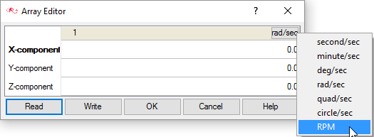
Click the Open Array button next to Angular velocity. In
the dialog box that opens,
Change the unit selector to RPM.
Figure 15.
Enter 400 in the Y-component row.
Click OK to close the dialog.
Set the Multiplier function to MRF_Multiplier, which is
the function you created in the previous steps.
As the simulation progresses, the value of the rpm for the reference frame,
i.e. 400 rpm, will be multiplied with the instantaneous value of the multiplier
provided by the MRF_Multiplier function at every time step. Thus at time zero,
when the multiplier function evaluates to 1, the disc rpm will be 400. The rpm
will linearly decrease to zero over the next 2.8 seconds, before rising again to
400 and so on as per the multiplier.
Apply Volume Parameters
Volume groups are containers used for storing information about a volume region. This
information includes the list of geometric volumes associated with the container, as
well as attributes such as material models and mesh size information.
When the geometry was imported into AcuConsole, all
volumes were placed into the "default" volume container.
In the next steps you will create volume groups for each volume in the model, assign
volumes to the respective volume groups, rename the default volume group container,
and set the materials and other properties for each volume group.
In the process of setting up a simulation, you need to move into different panels for
setting up the material models, boundary conditions, mesh parameters, etc. which can
sometimes be cumbersome, especially for models with too many surfaces. To make it
easier, less error prone, and time saving, two new dialogs are provided in AcuConsole which you can use to verify and provide the
information for all surface or volume entities at once. They are the
Volume Manager and Surface Manager. In
this section some features of Volume Manager are exploited.
Click BAS in the Data Tree Manager to switch to basic view in the Data Tree.
Expand the ModelData Tree item.
Turn off the display of surfaces by right-clicking on
Surfaces and clicking Display
off in the context menu.
Expand Volumes. Toggle the display of the default
volume container by clicking
and next to the volume name.
Note: You may not see any change when toggling the display if
Surfaces are being displayed, as surfaces and
volumes may overlap.
Right-click on Volumes and select Volume
Manager.
In the Volume Manager Dialog, click on
Columns, select Medium from
the list and click Ok.
Figure 16.
Click New twice to create two new volume groups.
Turn the display off for all volumes except the default volume.
Rename the default volume to disc, Volume 1 to
inner_air, and Volume 2 to
outer_air.
Set the Medium, Material Model, and the Reference Frame for the volume groups
as per the table shown below.
Figure 17.
Note: You may need to expand the dialog to view all the columns.
Assign the respective volumes to their volume groups.
Click Add to in the row belonging to
inner_air.
Select the volume as shown in the figure below and click
Done.
Figure 18.
Click Add to in the row belonging to outer_air,
select the volume as shown in the figure below and click
Done.
Figure 19.
When the geometry was loaded into AcuConsole, the complete geometry volume was placed in a default surface group.
That volume group was renamed to disc. At this point, all that is left
is the disc volume group, which makes up the rotor disc of the
brake.
Figure 20.
Close the Volume Manager Dialog.
Create Surface Groups and Apply Surface Parameters
Surface groups are containers used for storing information
about a surface, including solution and meshing parameters, and the corresponding
surface in the geometry that the parameters will apply to.
In the next steps you will define surface groups,
assign the appropriate settings for the different characteristics of the problem,
and add surfaces to the group containers.
In the previous section, you were introduced to the Volume
Manager, which is used to quickly verify and set the basic parameters
for the volume groups. In this section some features of Surface
Manager are exploited.
Turn-off the display of Volumes by right-clicking on
Volumes and selecting Display off
.
Expand Surfaces in the Data Tree
and toggle on the display of the default surface container.
Right-click on Surfaces and select Surface
Manager.
In the Surface Manager Dialog, click
New seven times to create seven new surface
groups.
If you cannot see the Simple BC Active and Simple BC Type columns, click on
Columns and select these two columns from the list
then click Ok.
Turn off the display for all the surfaces except for the default surface and
rename to default surface to disc_surf.
Rename the other surfaces and set the Simple BC Active and Simple BC Type
columns as per the table shown below.
Figure 21.
Assign the surfaces to their respective surface groups.
Click Add to in the row belong to
symm_air_2.
Select the two surfaces as shown in the figure below and click
Done.
Figure 22.
Click Add to in the row belong to
symm_disc_2.
Select the surface as shown in the figure below and click
Done.
Figure 23.
Assign the corresponding surfaces on the other side of the domain to
the groups symm_air_1 and symm_disc_1 respectively.
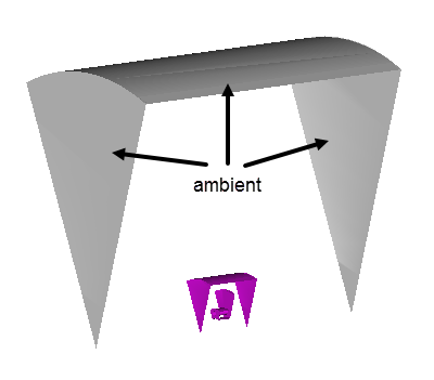
Assign the remaining peripheral surfaces of the geometry to the ambient
surface groups as shown in the figure below.
Figure 24.
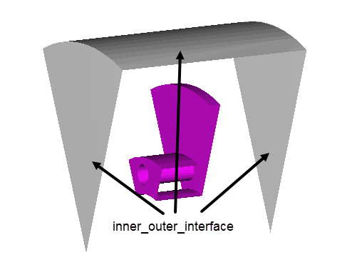
Assign the surfaces for inner_outer_interface. These are the surfaces
where the inner and the outer_air volume coincide. Note that these
surfaces will be overlapping with each other. One of these surface sets
will belong to the inner_air volume and the second to the outer_air
volume. Because of the overlap, you may need to repeat this step twice
for what may look like the same group of surfaces. However, these will
be two different surface sets.
Figure 25.
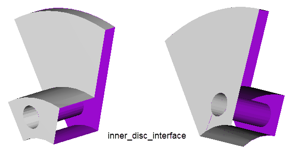
Assign the surfaces for inner_disc_interface. These are the surfaces
where the inner_air volume is in contact with the disc volume. Note that
these surfaces will be overlapping with another surface set belonging to
the disc volume. However, unlike the previous step, you only need to
select the surfaces on the inner_air volume side for this surface
group.
Figure 26.
When the geometry was loaded into AcuConsole, all geometry surfaces were placed in a default surface group. That
surface group was renamed to disc_surf. At this point, all that is left
is the disc_surf surface group, which makes up the bounding surfaces of
the disc volume.
Assign Surface Parameters (Boundary Conditions)
In next steps you will set boundary conditions for the surfaces that apply globally
to the simulation. To make this simple, the basic boundary conditions applicable for
any simulation can be filtered using the BC filter in the Data Tree Manager. However, for this tutorial you will also be using
some advanced capabilities of AcuConsole for specifying
the boundary conditions.
Click ALL in the Data Tree Manager to
display all the available options in the Data Tree.
Expand each of these surface groups in the Data Tree
and ensure that the Surface Boundary Condition option is not activated.
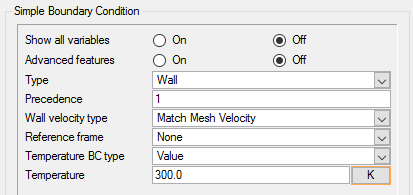
ambient
Expand the ambient surface group in the Data Tree.
Double-click Simple Boundary Condition to open the
boundary condition detail panel.
Ensure that Type is set to Wall.
Change the Temperature BC type to Value.
Set the value for Temperature to 300 K.
Figure 27.
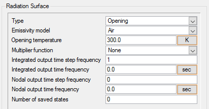
Double-click Radiation Surface under ambient to open the
radiation detail panel.
If you see the Activate flag set to off, switch it to
On.
Set the Type to Opening.
Set the Emissivity model to Air.
Set the Opening temperature to 300 K.
Figure 28.
disc_surf
Expand the disc_surf surface group in the Data Tree.
Check that the Surface Boundary Condition option is not active.
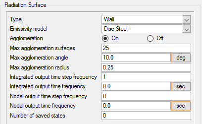
Double-click Radiation Surface under disc_surf to open
the radiation detail panel.
If you see the Activate flag set to off, switch it to
On.
Set the Type to Wall.
Set the Emissivity model to Disc Steel.
Accept all other default settings.
Figure 29.
Expand the Advanced Options tree under disc_surf.
Double-click Turbulence Wall to open the detail
panel.
If you see the Activate flag set to off, switch it to
On.
Set the Type to Wall Function.
Expand the Nodal Boundary Conditions tree under Advanced
Options.
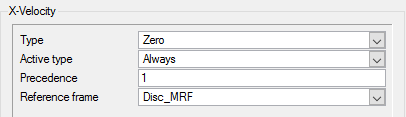
Double-click X-Velocity to open the detail panel.
If you see the Activate flag set to off, switch it to
On.
Set the Reference frame to Disc_MRF.
Figure 30.
Repeat the above three steps for Y and Z-Velocity.
Double-click Eddy Viscosity.
If you see the Activate flag set to off, switch it to
On. Leave the default settings.
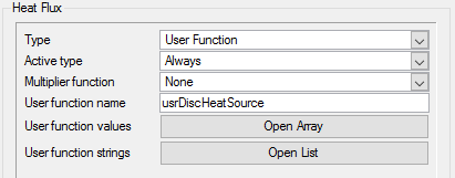
Apply Heat Transfer Parameters to the Disc
As discussed in the introduction, a user defined function will be used to define the
heat source on the disc. The script heatSource.c contains the
function usrDiscHeatSource, which will be used to assign heat flux on the disc
surface corresponding to the heat source due to braking. In addition, radiation heat
flux parameters will also be applied for the disc.
Expand the Element Boundary Conditions tree under
Advanced Options for the disc_surf surface group.
Double-click Heat Flux to open the detail panel.
If you see the Activate flag set to off, switch it to
On.
Set the Type to User Function.
For User function name, enter usrDiscHeatSource.
Figure 31.
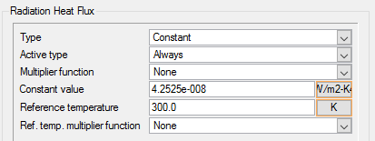
Double-click Radiation Heat Flux to open the detail
panel.
If you see the Activate flag set to off, switch it to
On.
Set the Type to Constant.
Set the Constant value to
4.2525e-008W/m2-K4.
Set the Reference temperature to 300 K.
Figure 32.
Set Periodic Boundary Conditions
The surface groups symm_air_1 and symm_air_2 are periodic surface groups with
axisymmetric periodicity along the axis of rotation of the disc. Similarly, surface
groups symm_disc_1 and symm_disc_2 are periodic as well. To ensure mesh conformity
between the periodic surface pairs, periodic boundary conditions should be defined
to pair the nodes before mesh is created. The mesh created thereafter will be
periodic.
Click BAS in the Data Tree Manager to switch to basic view in the Data Tree.
Right-click on Periodics in the Data Tree, and select New.
Repeat the previous step to create another entry, Periodic 2.
Rename Periodic 1 as periodicity_disc.
Rename Periodic 2 as periodicity_air.
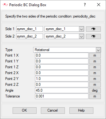
Right-click on periodicity_disc and select
Define.
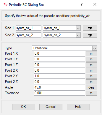
In the dialog that appears, set the following conditions:
Side 1: symm_disc_1
Side 2: symm_disc_2
Type: Rotational
Point 1 (x, y, z): (0, 0, 0)
Point 2 (x, y, z): (0, 1, 0)
Angle: 45 degrees
Tolerance: 0.001
Figure 33.
Similarly, define periodicity_air as shown below.
Figure 34.
Save the database to create a backup of your settings.
Define Nodal Outputs
The nodal output command specifies the nodal output parameters, for instance, output
frequency, number of saved states, etc.
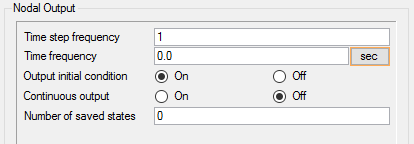
Expand the Output tree, then double-click
Nodal Output to open the Nodal
Output detail panel.
Set Time step frequency to 1.
This will save the nodal outputs at every time step.
Set Output initial condition to On.
This will instruct the solver to write the initial state of the problem as the
first output file.
Check that the Number of saved states option is set to zero.
Setting this option zero will instruct the solver to save all the solution
state files Figure 35.
.
Create a Time History Output Point
Time history output commands enable you to extract the nodal solution at any point
within the domain. In this simulation, it would be interesting to observe the
temperature of a point on the disc within the pad contact area as the brake is
applied and released.
Expand the Output tree, right-click on Time
History Output, and select New.
Rename Time History Output 1 to MonitorPoint.
Don't forget to press Enter after typing in the new
entity name.
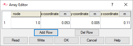
Double-click MonitorPoint. In the detail panel,
Change the Type to Coordinates.
Click Open Array next to Coordinates and edit
the values in the Array Editor according to the
image shown below.
Figure 36.
Set the Time step frequency to 1.
This will save the results for the defined time history point at every
time step.
Save the database to create a backup of your settings.
Assign Mesh Controls
Set Global Mesh Attributes
Now that the flow characteristics have been set for the whole problem, a sufficiently
refined mesh has to be generated.
Global mesh attributes are the meshing parameters applied to the model as a whole
without reference to a specific geometric volume, surface, edge, or point. Local
mesh attributes are used to create mesh generation controls for specific geometry
components of the model.
In the next steps you will set the global mesh attributes.
Click MSH in the Data Tree Manager to filter the
settings in the Data Tree to show only the controls
related to meshing.
Double-click the GlobalData Tree item to expand it.
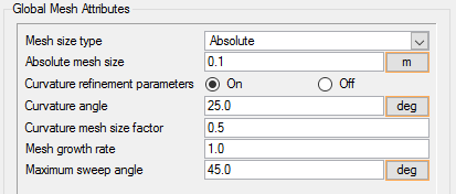
Double-click Global Mesh
Attributes to open the Global Mesh
Attributes detail panel.
Change the Mesh size type to Absolute.
Enter 0.1 for the Absolute mesh size.
Figure 37.
Set Surface Mesh Parameters
Surface mesh attributes are applied to a specific surface in the model. It is a
type of local meshing parameter used to create targeted mesh controls for one or
more specific surfaces.
Setting local mesh attributes, such as surface mesh attributes, is not mandatory.
When a local mesh attribute is not found for a component, the global attributes
are used as the mesh generation control for that component. If a local mesh
attribute is present, it will take precedence over the global setting.
In the next steps you will set the surface meshing attributes.
Expand the ModelData Tree item and then expand
Surfaces.
Expand the inner_disc_interface surface group under
Surfaces.
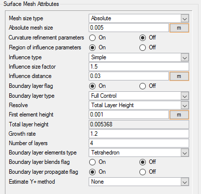
Double-click Surface Mesh Attributes under
inner_disc_interface to open the Surface Mesh Attributes
detail panel.
If you see the Activate flag set to off, switch it to
On.
Ensure that the Mesh size type is set to Absolute.
Enter 0.005 m for the Absolute mesh size.
Switch the Region of influence parameters flag to
On.
Region of influence is a size control that allows you to control the size and
growth rate of the surface and volume mesh surrounding a surface based on
the distance from the surface.
Set the Influence size factor to 1.5.
Set the Influence distance to 0.03.
Switch the Boundary layer flag to On.
Check the Boundary layer type is set to Full Control.
Set Resolve to Total Layer Height.
This will set the total layer height based on the other settings you
provide.
Set the remaining settings as follows:
First element height:
0.001
Growth rate:
1.2
Number of layers: 4
Boundary layer elements type: Tetrahedron
Set the Boundary layer propagate flag to On.
Figure 38.
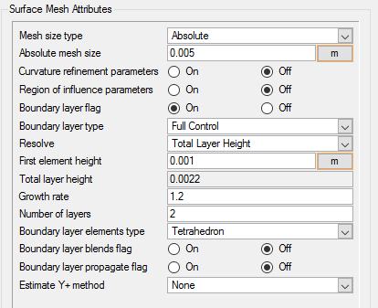
Similarly, set the Surface Mesh Attributes for disc_surf using the parameters
shown below.
Figure 39.
Generate the Mesh
In the next steps you will generate the mesh that will be used when computing a
solution for the problem.
Click on the toolbar to open the Launch
AcuMeshSim dialog.
For this case, the default settings will be used.
Click Ok to begin meshing.
During meshing an AcuTail window opens. Meshing
progress is reported in this window. A summary of the meshing process indicates that the
mesh has been generated.
Figure 40.
Note: The actual number of nodes and elements, and memory usage may vary
slightly from machine to machine.
Visualize the mesh in the modeling window. Turn on
the display of surfaces and set the display type to solid and
wire.
Rotate and zoom in the model to analyze the various mesh regions.
Compute the Solution and Review the Results
Set Initial Conditions
As mentioned in an earlier section, results from the precursor simulation will be
used to define the initial conditions for this case. The projection of the available
results on the current mesh will be done using the AcuProj utility in the following
steps.
Select Tools > Project Solution from the menu bar.
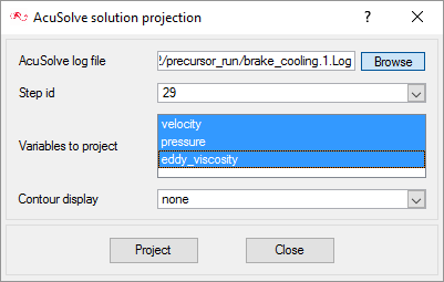
In the AcuSolve solution projection dialog that opens,
click Browse next to the AcuSolve log
file field.
Navigate to the precursor_run directory containing the
solution to be projected.
Select brake_cooling.1.Log from the directory.
Click Open.
Verify that the Step id is 29 in the AcuSolve solution
projection dialog.
Select all the variables available in the Variables to project field (velocity,
pressure, and eddy_viscosity).
You may need to hold Shift while clicking the top and
bottom of the list to select all the variables. Figure 41.
Click Project, then click
Close.
The above setups will set the initial conditions for the pressure, velocity
and the eddy viscosity fields. Since the precursor run does not has the
temperature field data, it needs to be set manually.
Click BAS in the Data Tree Manager to switch to basic view in the Data Tree.
Double-click on Nodal Initial Condition under Global in
the Data Tree.
In the detail panel, set the Temperature initial condition type to
Constant and the Temperature to
300 K.
Save the database to create a backup of your settings.
Compile the UDF
A UDF written in C language (heatSource.c) is provided with
the tutorial. This C source file should now be compiled using the following
steps.
The utilities required for compiling are different on Windows and
Unix operating systems. Follow the steps below according
to your machine
Compiling the UDF for Windows:
Start AcuSolve Command Prompt from the
Windows Start menu by clicking Start > All Programs > Altair HyperWorks <version> > AcuSolve > AcuSolve Cmd Prompt.
Change the directory to the present working directory using the
cd command.
Enter the following command at the prompt:
acuMakeDll –src heatSource.c
Compiling the UDF for Unix operating system:
In the terminal, use the cd command to change the
directory to the current working directory.
Note: If you open a new terminal, please source the AcuSolve build before proceeding.
Enter the following command at the prompt:
acuMakeLib –src heatSource.c
Once the compilation is complete, a set of files necessary for AcuSolve to read and process the UDF will be created.
Run AcuSolve
In the next steps you will launch AcuSolve to compute the solution for this case.
Click on the toolbar to open the
Launch AcuSolve dialog.
Click Ok to start the
solution process.
While computing the solution, an
AcuTail window opens. Solution progress is
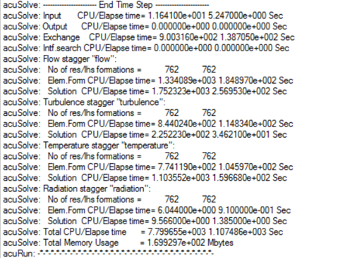
reported in this window. A summary of the solution process indicates
that the run has been completed.
The information provided in the summary is based on
the number of processors used by AcuSolve.
If you use a different number of processors than indicated in this
tutorial, the summary for your run may be slightly different than the
summary shown.
Figure 42.
Close the AcuTail window and save the database to create a
backup of your settings.
Post-Process with AcuProbe
AcuProbe can be used to monitor various variables over
solution time.
Open AcuProbe by clicking on the toolbar.
In the Data Tree on the left, expand Time History > MonitorPoint > node 1.
Right-click on temperature and select
Plot.
This will plot the temperature of the point which you defined as the time
history output point as the solution progresses.
Note: You might need to click on the toolbar in order to
properly display the plot.
Figure 43.
The temperature profile of the monitor point follows the expected
behaviour. It can be seen that the disc does not cool down completely before
the next braking cycle starts, and thus the maximum temperature reached
increases with every following cycle.
You can also save the plots as an image.
From the AcuProbe dialog, click File > Save.
Enter a name for the image and click
Save.
The time series data of the variables can also be exported as a text file
for further post-processing.
Right-click on the variable that you want to export and click
Export.
Enter a File name and choose .txt for
the Save as type.
Click Save.
View Results with AcuFieldView
Prerequisites
The tutorial has been written with the assumption that you have become familiar with
the AcuFieldView interface and basic operations. In
general, it will be helpful to understand the following basics:
How to find the data readers in the File pull-down on the Main menu and open the
desired reader panel for data input.
How to find the visualization panels, either from the Side toolbar or the
Visualization panel pull-downs on the Main menu, and create and modify surfaces
in AcuFieldView.
How to move the data around the graphics window using mouse actions to
translate, rotate and zoom in to the data.
This tutorial shows you how to work with transient analysis data.
Launch AcuFieldView
Click on the
AcuConsole toolbar to open the
Launch AcuFieldView dialog.
Click Ok to start
AcuFieldView.
You will see that the temperature contours
have already been displayed on all the boundary surfaces with mesh. When you
start AcuFieldView from AcuConsole, the results from the last time step of
the solution that were written to disk will be loaded for post-processing.
Set Up AcuFieldView
Close the Boundary Surface dialog.
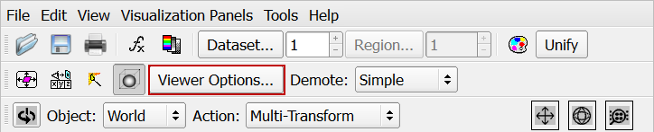
Click Viewer Options.
Figure 44.
In the Viewer Options dialog:
Deselect Perspective to turn off the perspective
view.
Click Axis Markers to disable the axis markers.
Click Close.
On the toolbar, click the Colormap icon .
In the Scalar Colormap Specification dialog, click
Background and select White.
Close the Scalar Colormap Specification dialog.
Click the Toggle Outline icon on the toolbar to turn off the outline display.
Your display should now look like this. Figure 45.
Visualize and Save an Animation of the Temperature Variation with Time
Click to open the Boundary
Surface dialog.
From the Boundary Types panel, select OSF: disc_surf and
click OK.
Change the Coloring to Scalar.
Change the Display Type to Smooth.
Deactivate the Show Mesh check box.
From the toolbar, click to open the Defined
Views dialog.
Select -Y then click Close.
In the Colormap tab of the Boundary Surface dialog,
activate the Local check box.
In the Legend tab, check the Show Legend check
box.
Change the Label color to black.
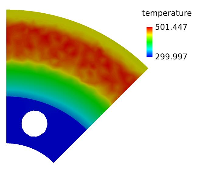
Your display should now look like this. The visible temperature profile
on the disc surface is the profile at the end of last time step in the
simulation.
Note: You may need to adjust the zoom level and pan the model to
get the view shown below.
Figure 46.
Close the Boundary Surface dialog.
From the Tools menu, select Flipbook Build Mode. In the
Flipbook Size Warning window, click OK.
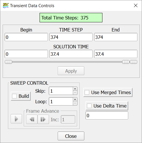
Go to the Tools menu again and select Transient
Data.
This will open the Transient Data Controls dialog.
Figure 47.
If the Sweep Control in this dialog says Sweep instead of Build, the
Flipbook Build Mode is not active. In Sweep mode, you will be able to create
and visualize the animation but you will not be able to save it. To be able
to save the animation, enable the Flipbook Build Mode.
Drag the time step slider to its leftmost position. Alternatively, enter
0 in the Time Step or Solution Time box. Click
Apply.
The displayed state now corresponds to the initial state of the domain, as
defined by the projected solution from the precursor_run directory used for
initializing this setup. Since the projected solution did not include
temperature data, and temperature initial condition was a constant value. That
is what you see here.
Click Build.
AcuFieldView will now build the
frame-by-frame animation of the solution progressing through all the available
time steps. You will be able to see the progress in a Building
Flipbook dialog. Once the build process is complete, a
Flipbook Controls dialog will appear.
Click to play the animation.
As the animation progresses, you will be able to see the variation of
temperature on the disc surface with time. The temperature increases while the
brake is pressed, and once the brake is released, the disc slowly cools down
before the brake is applied again. Then the whole cycle repeats itself.
To save the animation, click , then click Save.
Summary
In this AcuSolve tutorial, you successfully set up and solved a disc
brake simulation problem. You started the tutorial by creating a database in AcuConsole, setting up the simulation parameters, importing, and
meshing the geometry. A moving reference frame approach along with a multiplier function
was used to model the brake-release cycle in a vehicle. Once the case was setup, the
solution was generated with AcuSolve. AcuProbe was used to visualize the variation of temperature on a
monitor point on the disc surface during the simulation. AcuFieldView was then utilized to generate an animation of the
temperature profile on the disc during the simulation.

 on the toolbar.
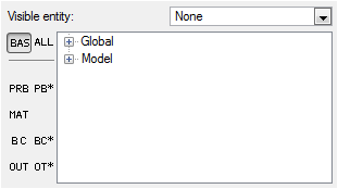
 next to the item name.
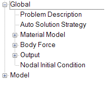
 on
the toolbar.
on
the toolbar.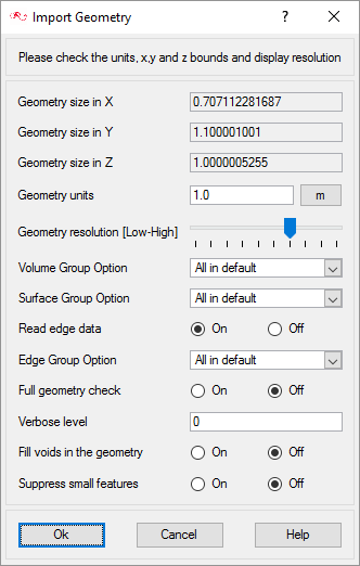
 and
and  next to the volume name.
Note: You may not see any change when toggling the display if Surfaces are being displayed, as surfaces and volumes may overlap.
next to the volume name.
Note: You may not see any change when toggling the display if Surfaces are being displayed, as surfaces and volumes may overlap.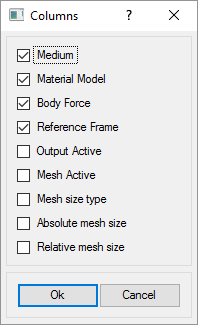
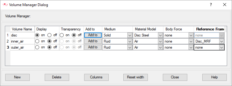
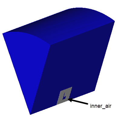
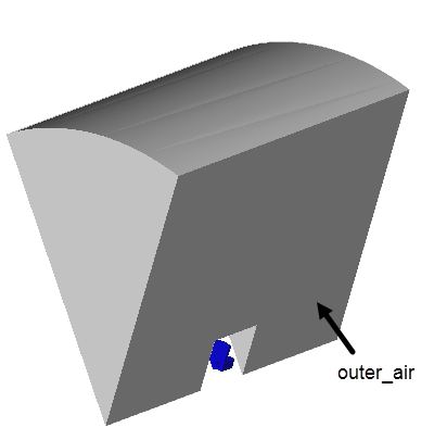
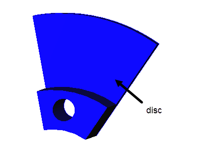
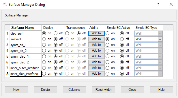
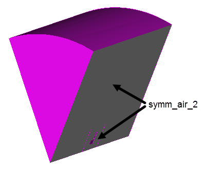 Figure 22.
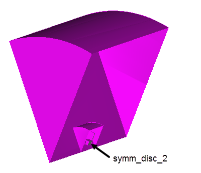
 on the toolbar to open the Launch
AcuMeshSim dialog.
For this case, the default settings will be used.
on the toolbar to open the Launch
AcuMeshSim dialog.
For this case, the default settings will be used.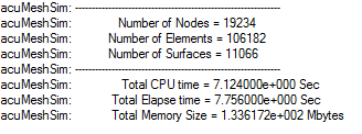
 on the toolbar to open the
Launch AcuSolve dialog.
on the toolbar to open the
Launch AcuSolve dialog.
 on the toolbar.
 on the toolbar in order to
properly display the plot.
on the toolbar in order to
properly display the plot.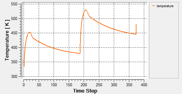
 on the
AcuConsole toolbar to open the
Launch AcuFieldView dialog.
on the
AcuConsole toolbar to open the
Launch AcuFieldView dialog.
 .
.
 on the toolbar to turn off the outline display.
Your display should now look like this.
on the toolbar to turn off the outline display.
Your display should now look like this.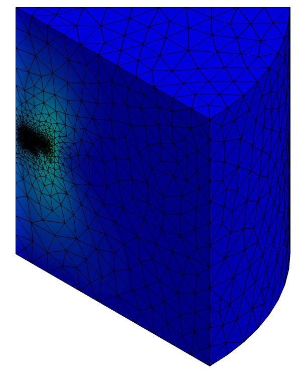
 to open the Boundary
Surface dialog.
to open the Boundary
Surface dialog.
 to open the Defined
Views dialog.
to open the Defined
Views dialog.
 to play the animation.
As the animation progresses, you will be able to see the variation of temperature on the disc surface with time. The temperature increases while the brake is pressed, and once the brake is released, the disc slowly cools down before the brake is applied again. Then the whole cycle repeats itself.
to play the animation.
As the animation progresses, you will be able to see the variation of temperature on the disc surface with time. The temperature increases while the brake is pressed, and once the brake is released, the disc slowly cools down before the brake is applied again. Then the whole cycle repeats itself. , then click Save.