ACU-T: 5001 Blower - Transient (Sliding Mesh)
Prerequisites
This tutorial provides the instructions for setting up, solving, and viewing results for a transient simulation of a centrifugal air blower utilizing the sliding mesh approach. In order to run this tutorial, you should have already run through ACU-T: 5000 Blower - Steady (Rotating Frame) and kept the solution in your working directory. It is assumed that you have some familiarity with HyperWorks CFD and AcuSolve. To run this simulation, you will need access to a licensed version of HyperWorks CFD and AcuSolve.
Prior to running through this tutorial, copy HyperWorksCFD_tutorial_inputs.zip from <Altair_installation_directory>\hwcfdsolvers\acusolve\win64\model_files\tutorials\AcuSolve to a local directory. Extract ACU-T5001_BlowerTransient.hm from HyperWorksCFD_tutorial_inputs.zip.
Since the HyperWorks CFD database (.hm file) uses the ACU-T:5000 Blower-Steady model, this tutorial skips the geometry clean-up and inlet boundary conditions as well as the mesh settings.
Problem Description
The model consists of a centrifugal blower with a wheel of backward curved blades, and a housing with inlet and outlet ducts.

Figure 1. Schematic of Centrifugal Blower
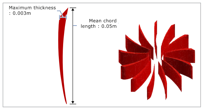
Figure 2. Schematic of Fan Blades
Start HyperWorks CFD and Open the HyperMesh Database
-
From the Home tools, Files tool group, click the Open Model tool.

Figure 3.The Open File dialog opens.
Set Up Flow
Set Up the Simulation Parameters and Solver Settings
-
From the Flow ribbon, click the Physics tool.

Figure 4.The Setup dialog opens. -
Under the Physics models settings:
- Set Time marching to Transient.
- Set the Time step size to 0.0005 and the Final time to 0.05.
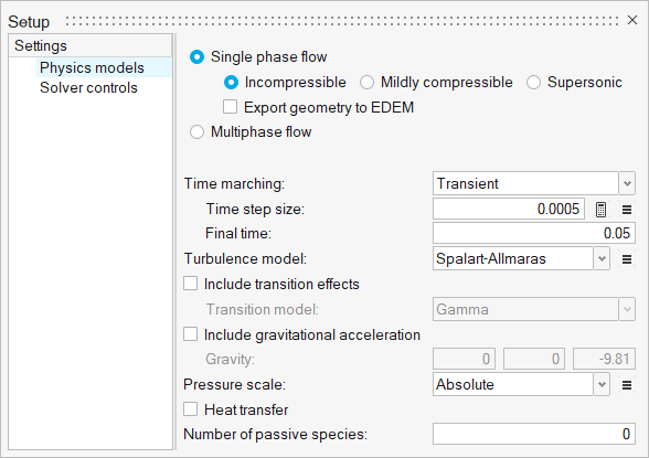
Figure 5. -
Set the Minimum stagger iterations and Maximum stagger iterations to
2 and 6, respectively.
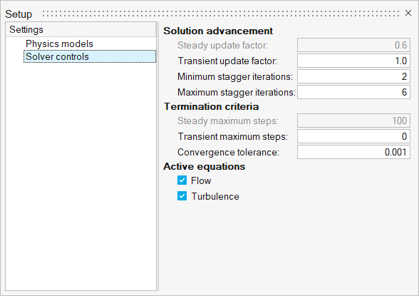
Figure 6.
Define Flow Boundary Conditions
-
From the Flow ribbon, Pressure
tool group, click the Stagnation Pressure tool.

Figure 7. -
Click the face of the inlet.
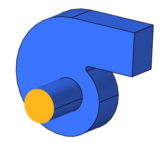
Figure 8. -
Set the Turbulence flow type to Internal.
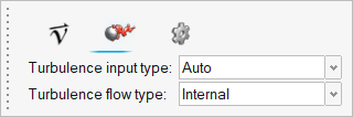
Figure 9. -
On the guide bar, click
 to execute
the command and exit the tool.
to execute
the command and exit the tool.
-
Click the Outlet tool.

Figure 10. -
Click the face of the outlet.
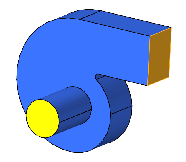
Figure 11. -
In the microdialog, make sure both Static pressure and Pressure loss
factor are 0.
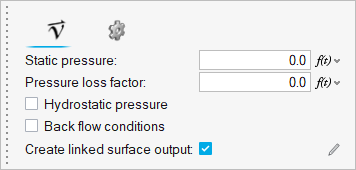
Figure 12. -
On the guide bar, click
to execute
the command and exit the tool.
Set Up Mesh Motion
Define the Mesh Motion Type
-
From the Motion ribbon, click the Settings tool.
Figure 13.The Setup dialog opens.
Define the Rotating Mesh Motion
-
Hide the housing solid.
- Set the entity selector to Solids.
- Select the centrifugal housing.
- Right-click and select Hide or press H on your keyboard.
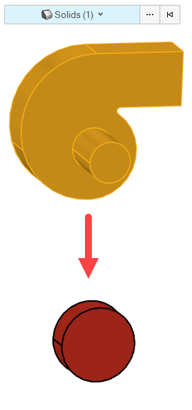
Figure 14. -
Click the Rotation tool.

Figure 15. -
Define the axis of rotation.
-
Use the Surf Center snap point to place the axis in the middle of the
centrifugal blower.
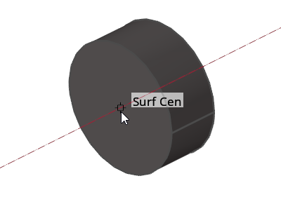
Figure 16. -
Click
 to change the rotational direction.
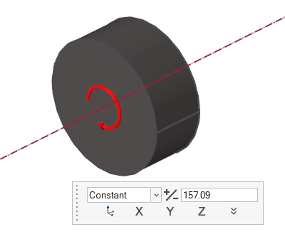
Figure 17. -
Use the Surf Center snap point to place the axis in the middle of the
centrifugal blower.
-
On the guide bar, click
to execute
the command and exit the tool.
Define Nodal Output Frequency
-
From the Solution ribbon, click the Field tool.

Figure 18.The Field Output dialog opens. -
Set the Time step interval to 1.
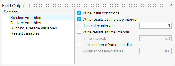
Figure 19.
Run AcuSolve
-
From the Solution ribbon, click the Run tool.

Figure 20. -
Leave the remaining options as default and click
Run to launch AcuSolve.
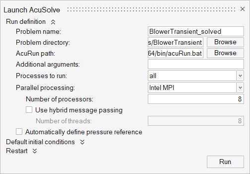
Figure 21.Tip: While AcuSolve is running, right-click on the AcuSolve job in the Run Status dialog and select View Log File to monitor the solution process.
Plot Surface Output
-
Right-click on the AcuSolve run in the
Run Status dialog and select Plot time
history.
The plot utility shows the residuals of the equations as the solution progresses through each time step.
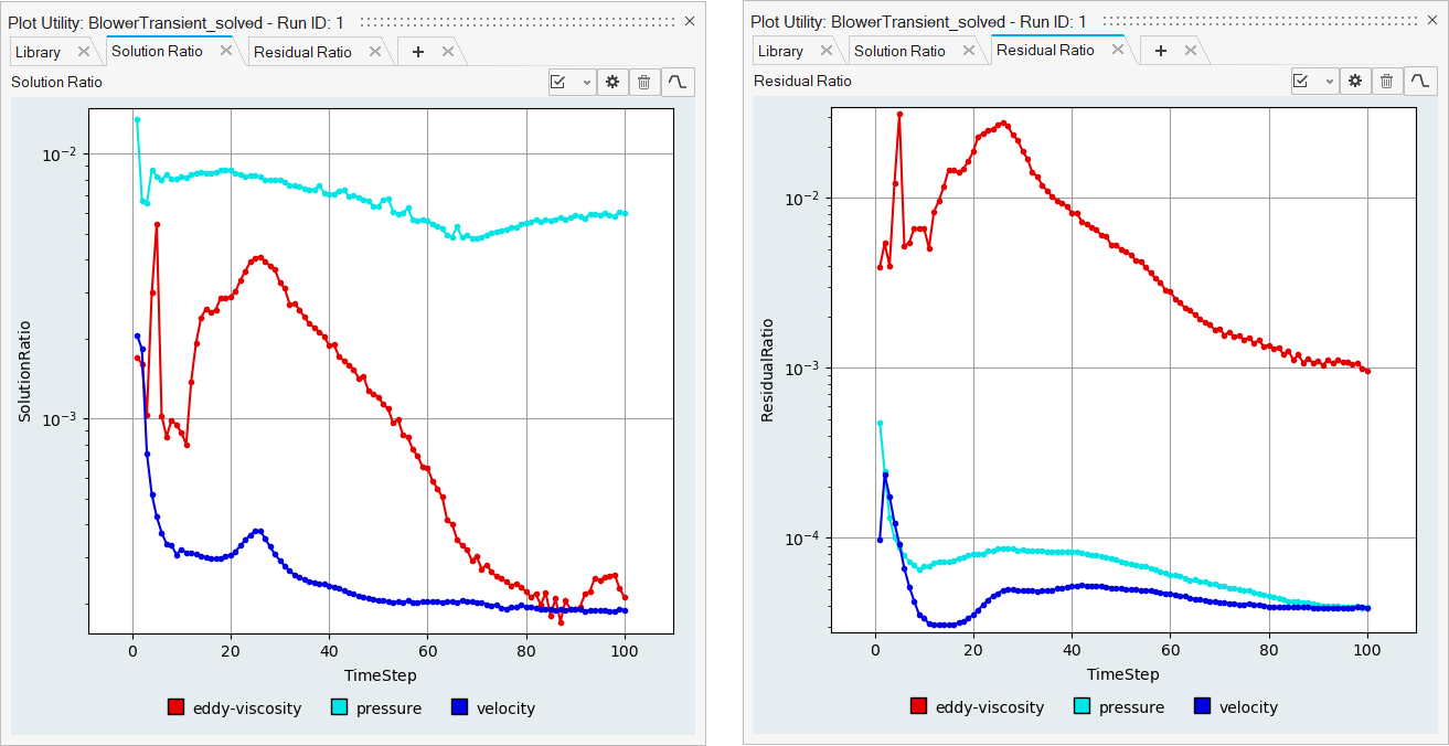
Figure 22. -
Click
 to add a new plot.
-
Under the Y-Axis heading, click the arrow besides Run
Data and select Surface Output
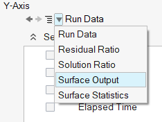
Figure 23. -
Select blades for the surface output.
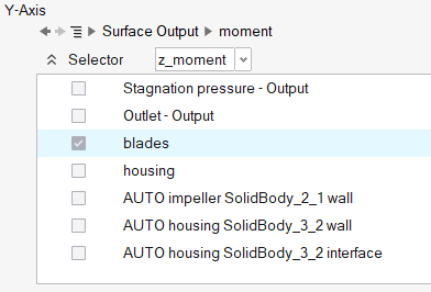
Figure 24. -
Click Create.
Figure 25.
Post-Process the Results with HW-CFD Post
-
Click the Slice Planes tool.

Figure 26. -
In the microdialog, click
 and move the plane along its normal direction a distance of
-0.07.
and move the plane along its normal direction a distance of
-0.07.
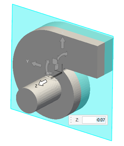
Figure 27. -
In the slice plane microdialog, click
 to create the slice plane.
-
Click
 and set the Colormap Name to Rainbow
Uniform.
and set the Colormap Name to Rainbow
Uniform.
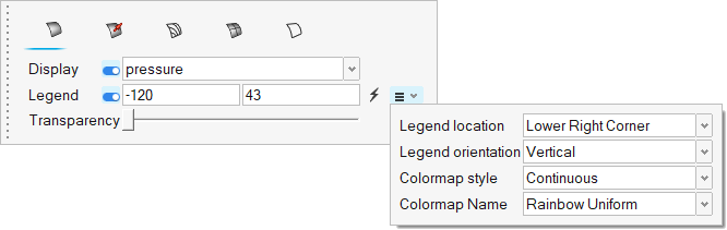
Figure 28. -
On the guide bar, click
to execute
the command and exit the tool.
-
Click the play button on the Animation toolbar.
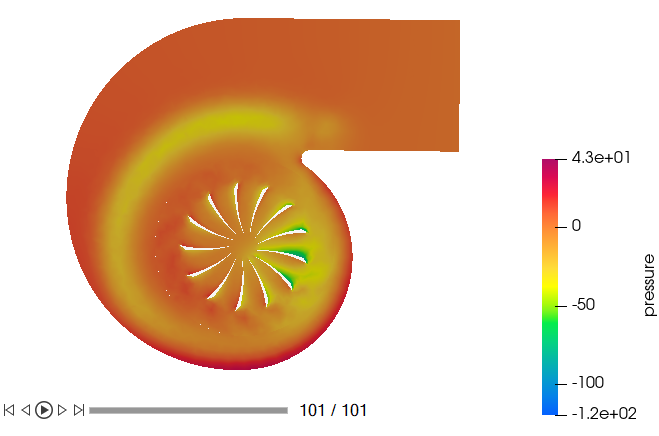
Figure 29.
Summary
In this tutorial, you worked through a basic workflow to set up a transient simulation with a sliding mesh in a centrifugal blower. You started by importing the mesh; once the case was set up, you generated a solution using AcuSolve. Then, you computed the blower momentum using the Plot Utility and created a contour plot for pressure on a cut plane using HW-CFD post.