ACU-T: 4201 Condensation & Evaporation - Air Box
Prerequisites
This tutorial provides instructions for running a transient simulation of an enclosed air-box using the humidity model. Prior to starting this tutorial, you should have already run through the introductory HyperWorks tutorial, ACU-T: 1000 HyperWorks UI Introduction, and have a basic understanding of HyperWorks CFD and AcuSolve. To run this simulation, you will need access to a licensed version of HyperWorks CFD and AcuSolve.
Prior to running through this tutorial, copy HyperWorksCFD_tutorial_inputs.zip from <Altair_installation_directory>\hwcfdsolvers\acusolve\win64\model_files\tutorials\AcuSolve to a local directory. Extract ACU-T4201_Air_Box.hm from HyperWorksCFD_tutorial_inputs.zip.
Problem Description

Figure 1.
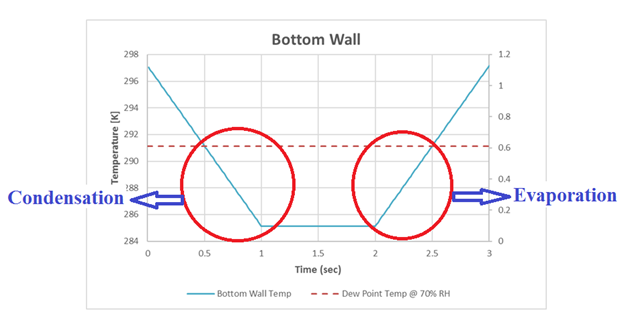
Figure 2.
From the above plot, we can see that the Air volume initial temperature is set to 297.15 K. The Bottom Wall temperature drops to 285.13 K over 1 sec, maintains 285.13 K for 1 sec, and then rises back to 297.15 K over 1 sec. The dew point temperature of the air at 70% RH is 291.14 K and is reached at 0.5 and 2.5 sec. On the whole we can see that both condensation and evaporation occurs when the dew point temperature is reached, as explained above.
Start HyperWorks CFD and Open the HyperMesh Database
-
From the Home tools, Files tool group, click the Open Model tool.

Figure 3.The Open File dialog opens.
Validate the Geometry
The Validate tool scans through the entire model, performs checks on the surfaces and solids, and flags any defects in the geometry, such as free edges, closed shells, intersections, duplicates, and slivers.
Figure 4.
Set Up Flow
Set Up the Simulation Parameters and Solver Settings
-
From the Flow ribbon, click the Physics tool.

Figure 5.The Setup dialog opens. -
Under the Physics models setting:
- Select the Multiphase flow radio button.
- Set the Multifluid type to Humidity transport.
- Set the Time step size to 0.1 s and the Final time to 10 s.
- Set the Turbulence model to Spalart-Allmaras.
- Set the Gravity to (0,-9.81,0).
-
Set the Pressure scale to Gauge and click
 . In the microdialog, set the Absolute pressure offset to 101325 Pa
then press Esc.
. In the microdialog, set the Absolute pressure offset to 101325 Pa
then press Esc.
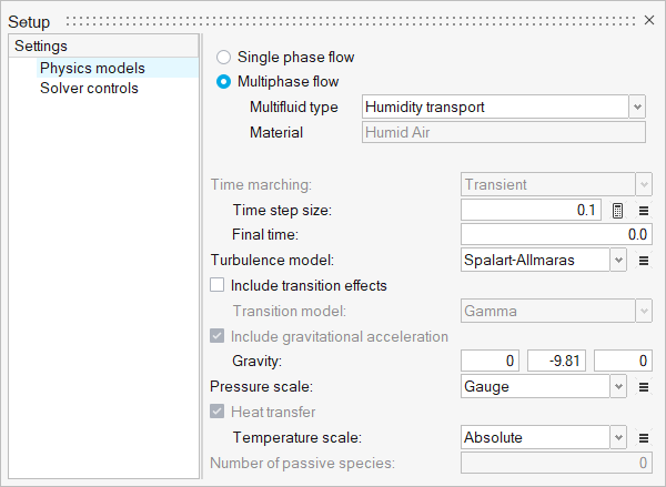
Figure 6. -
Set the Minimum stagger iterations to 2 and the Maximum
to 4.
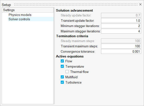
Figure 7.
Define Flow Boundary Conditions
-
From the Flow ribbon, click the No Slip tool.

Figure 8. -
Select the bottom surface (the surface with the minimum y-coordinate).
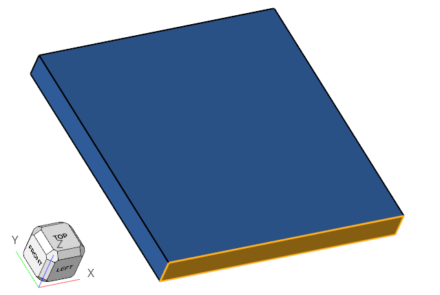
Figure 9. -
Set the Temperature to 1, expand the multiplier function
drop-down, and select Create new.
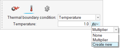
Figure 10. -
Click
 twice to add two rows.
-
Enter the values as shown in the figure below then close the dialog.
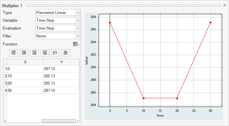
Figure 11. -
On the guide bar, click
 to execute
the command and exit the tool.
to execute
the command and exit the tool.
-
Click the Slip tool.

Figure 12. -
Select the surface with the maximum z-coordinate.
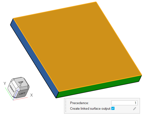
Figure 13. -
On the guide bar, click
 to execute the command and remain in the
tool.
to execute the command and remain in the
tool.
-
Select the surface with the minimum z-coordinate.
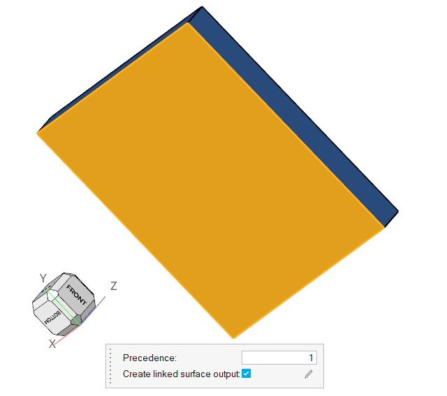
Figure 14. -
Click
 on the guide bar.
Compute the Solution
The input HyperMesh database contains the mesh, hence you do not need to generate the mesh again.
Define the Nodal Initial Conditions
-
From the Solution ribbon, click the Part tool.

Figure 15. -
In the dialog, click
 , select Relative Humidity
from the list of variables then click on the white space in the dialog.
, select Relative Humidity
from the list of variables then click on the white space in the dialog.
-
Set the value to 70.
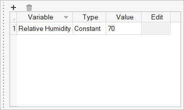
Figure 16. -
Click on the guide bar.
Run AcuSolve
-
From the Solution ribbon, click the Run tool.

Figure 17. -
Leave the remaining options as default and click
Run to launch AcuSolve.
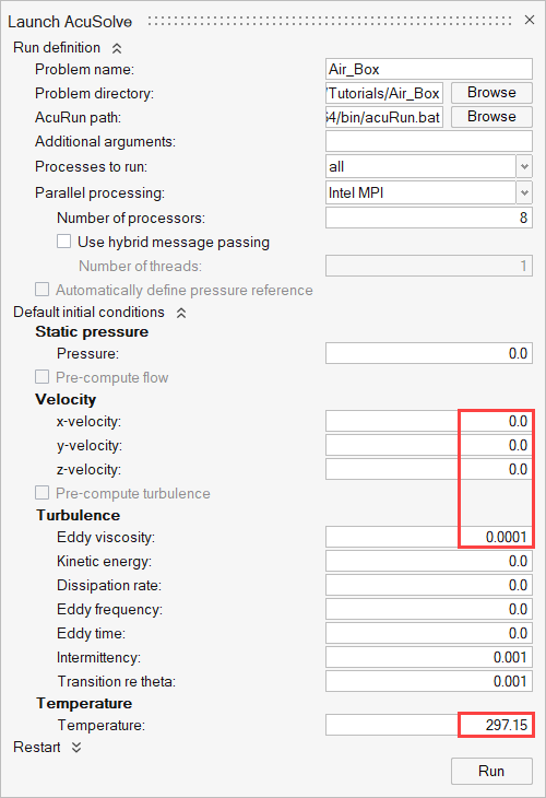
Figure 18.Tip: While AcuSolve is running, right-click on the AcuSolve job in the Run Status dialog and select View Log File to monitor the solution process. -
Click the Plot tool.

Figure 19. -
In the Plot Utility dialog, double-click on
Residual Ratio to plot the residuals.
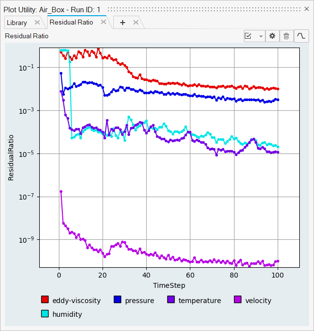
Figure 20. -
Click to add a new plot.
-
To set the Y-Axis variable, click
 and then double click on
temperature under Surface Output from the list of
variables.
and then double click on
temperature under Surface Output from the list of
variables.
-
In the list of surface outputs, select Bottom -
Output.
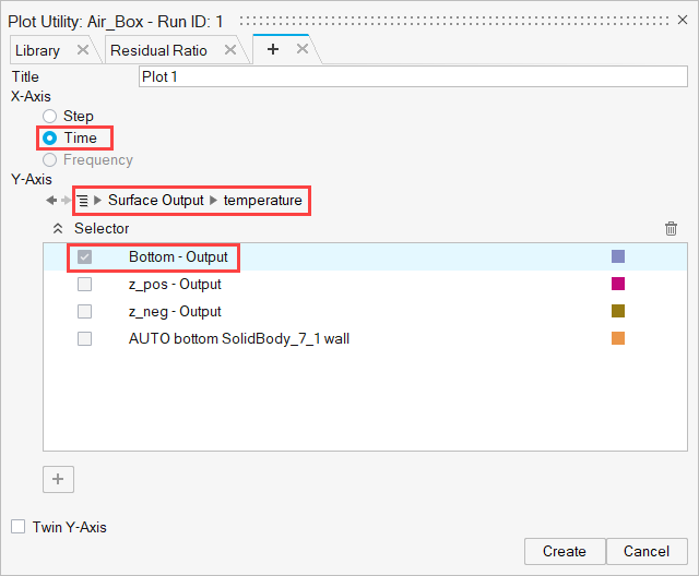
Figure 21. -
Click Create.
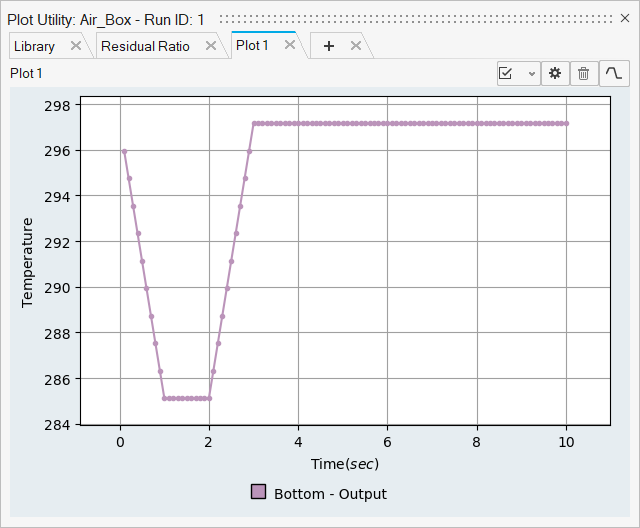
Figure 22. -
Similarly, view the plots for Relative Humidity and Dewpoint Temperature.
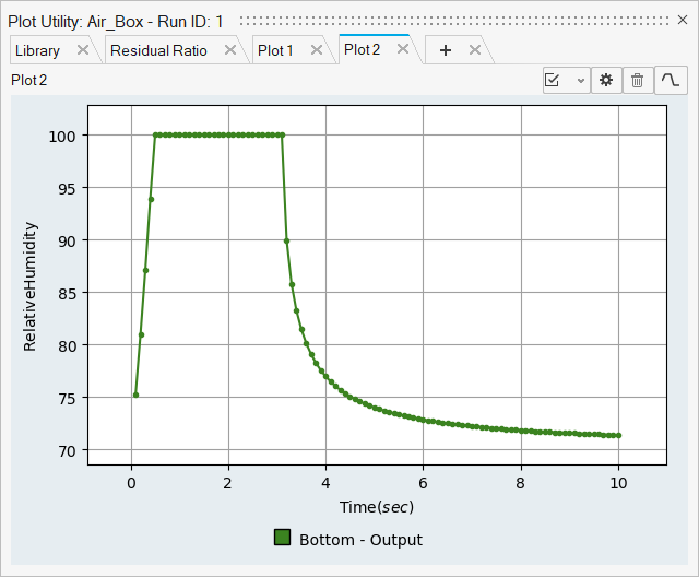
Figure 23.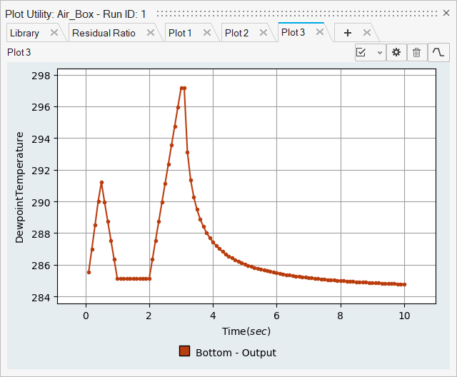
Figure 24.
Post-Process the Results with HW-CFD Post
In this step, you will create contour plots for temperature, relative humidity, and dew point temperature.
-
In the Post Browser, click on the icon beside
Flow Boundaries to turn off the display of all the
surfaces.
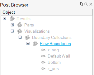
Figure 25. -
Drag the slider on the Animation toolbar to the 10th frame.

Figure 26. -
Click the Slice Planes tool.

Figure 27. -
Select the x-y plane in the modeling window.
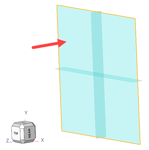
Figure 28. -
In the slice plane microdialog, click
 to create the slice plane.
-
Click
 then activate the Legend
toggle.
then activate the Legend
toggle.
-
Click
 and set the Colormap Name to Rainbow
Uniform.
and set the Colormap Name to Rainbow
Uniform.

Figure 29. -
On the guide bar, click to
create the temperature contour plot.
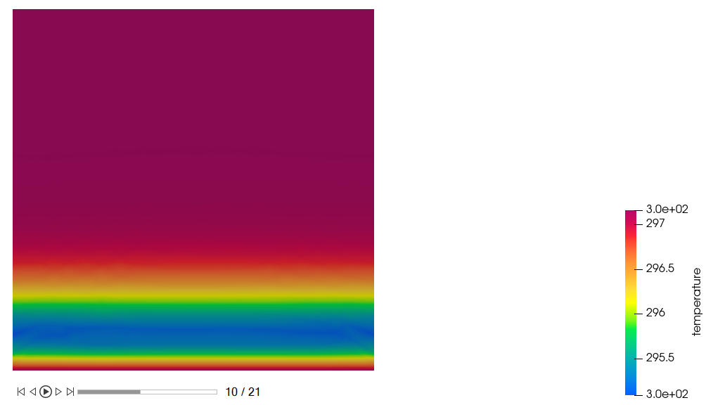
Figure 30. -
Hide the temperature contour, then repeat the steps 6-12 to create a similar
contour plot for relative humidity.
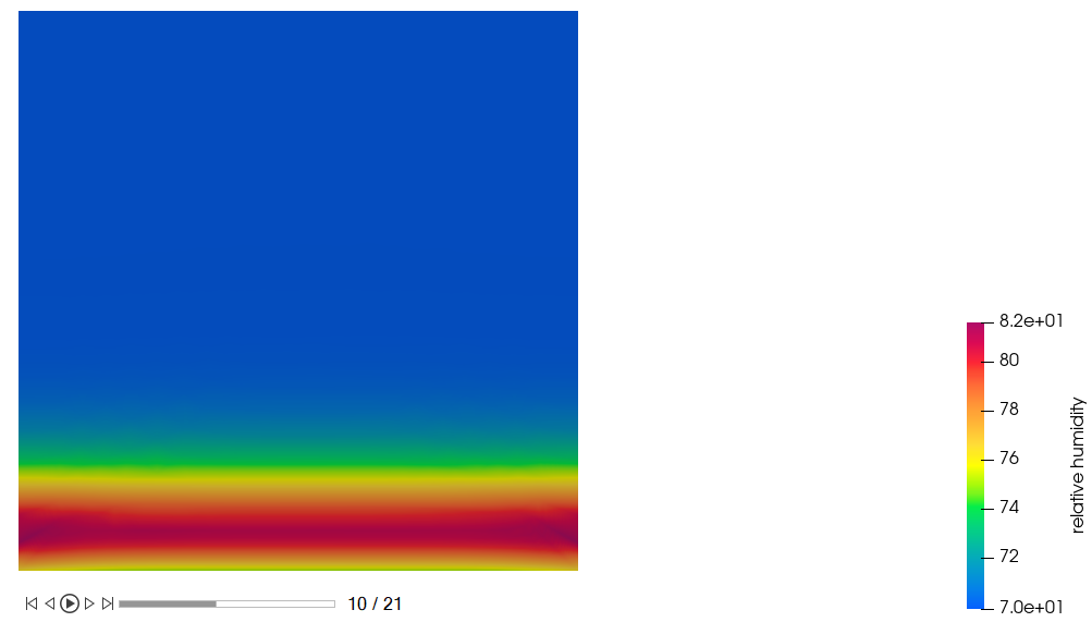
Figure 31. -
Hide the relative humidity contour, then repeat the steps 6-12 to create a
similar contour plot for dew point temperature.
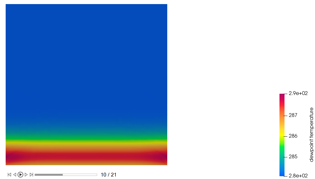
Figure 32.
Summary
In this tutorial, you learned how to set up and solve a multiphase humid air condensation and evaporation simulation using HyperWorks CFD and AcuSolve. You started by importing the HyperWorks CFD input database and then defined the flow setup. Once the solution was computed, you created a plot of residual ratios using the plot utility in HyperWorks CFD. Finally, you created a contour plot of temperature distribution, relative humidity, and dew point temperature using HyperWorks CFD Post.