ACU-T: 4100 Multiphase Flow using Algebraic Eulerian Model
Prerequisites
This tutorial provides instructions for running a transient simulation of a two-phase flow in a pipe using the Algebraic Eulerian model. Prior to starting this tutorial, you should have already run through the introductory HyperWorks tutorial, ACU-T: 1000 HyperWorks UI Introduction, and have a basic understanding of HyperWorks, AcuSolve, and HyperView. To run this simulation, you will need access to a licensed version of HyperMesh and AcuSolve.
Prior to running through this tutorial, copy HyperMesh_tutorial_inputs.zip from <Altair_installation_directory>\hwcfdsolvers\acusolve\win64\model_files\tutorials\AcuSolve to a local directory. Extract ACU-T4100_Disperse.hm from HyperMesh_tutorial_inputs.zip.
Since the HyperMesh database (.hm file) contains meshed geometry, this tutorial does not include steps related to geometry import and mesh generation.
Problem Description
The problem to be addressed in this tutorial is shown schematically in Figure 1. As an example, an LPipe problem is attached here to show the capability of the Disperse modeling in AcuSolve. The Algebraic Eulerian (AE) model is used to simulate the momentum exchange between a carrier field and a dispersed field. When simulating multiphase flows using the AE model, the carrier field has to be a fluid and the dispersed field can be of any medium.
In this problem, Water is considered a Carrier field material and Air is considered as Dispersed field material. Fluid enters the Inlet at an Average Velocity of 1 m/sec and the Water and Air volume fractions at the inlet are 96% and 4% respectively.
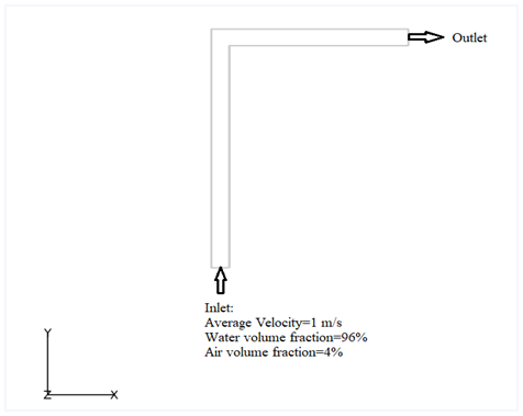
Figure 1.
Open the HyperMesh Model Database
-
Click the Open Model icon
 located on the standard toolbar.
The Open Model dialog opens.
located on the standard toolbar.
The Open Model dialog opens.
Set the General Simulation Parameters
Set the Analysis Parameters
-
Set Multiphase equation to Algebraic Equation.
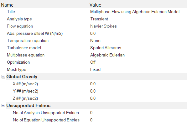
Figure 2.
Specify the Solver Settings
-
Verify that Flow, Turbulence, and Field are turned
On.
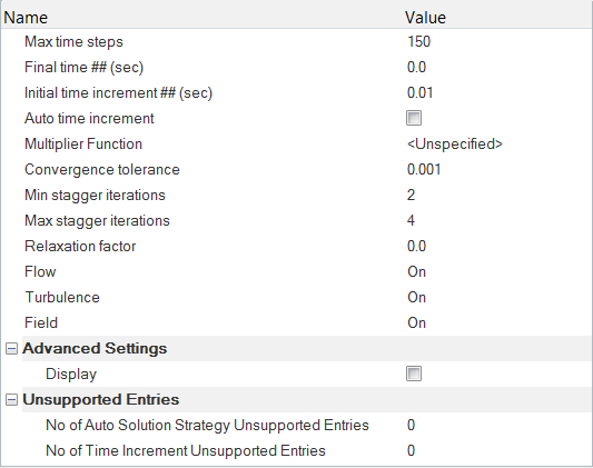
Figure 3.
Define the Nodal Outputs
-
Toggle On the Output initial condition field.
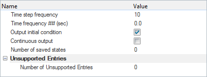
Figure 4.
Set Up Material Model Parameters and Body Force
In this step, you will start by setting up the Multiphase material model and body force parameters. Then, you will assign the surface boundary conditions and material properties to the fluid volume.
Set Up Material Model Parameters
-
Verify that the Number of Dispersed Field is set to
1.
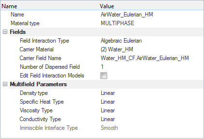
Figure 5. -
In the dialog, set the Dispersed Field 1 Material to
Air_HM, if not set already.
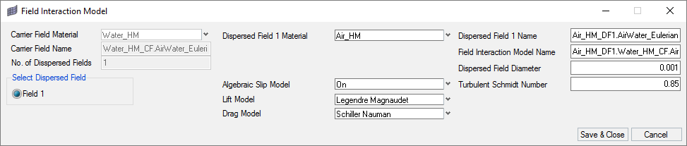
Figure 6.
Set Up the Body Force
-
In the Entity Editor, set the Z gravity to
0.0 and change the Y gravity to
-9.81 m/sec2.
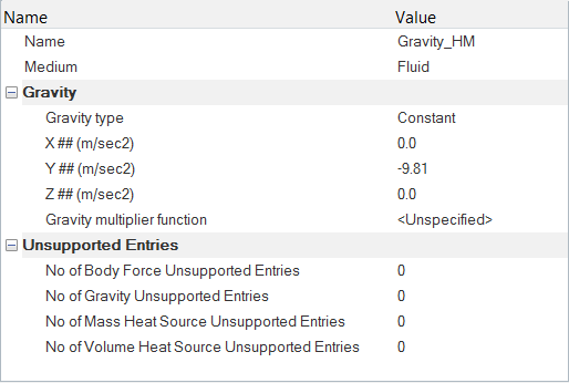
Figure 7.
Set Up Boundary Conditions and Nodal Initial Conditions
Assign Boundary Conditions and Material Properties
-
Click Fluid. In the Entity Editor,
- Change the Type to MULTIPHASE.
- Select AirWater_Eulerian_HM as the Material.
- Set Body force to Gravity_HM.
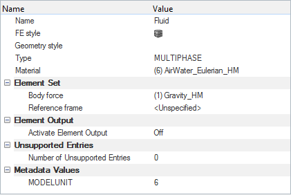
Figure 8. -
Click Inflow. In the Entity Editor,
-
Set No. of multiphase incoming fields to 2.0 and
press Enter on the keyboard.
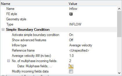
Figure 9.The Incoming Fields dialog opens. -
Select Water_HM_CF.AirWater_Eulerian_Hm as the
second Incoming Field and set Volume Fraction to
0.96.
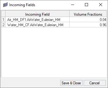
Figure 10.
-
Set No. of multiphase incoming fields to 2.0 and
press Enter on the keyboard.
-
Click Outflow. In the Entity Editor, change the Type to
OUTFLOW.
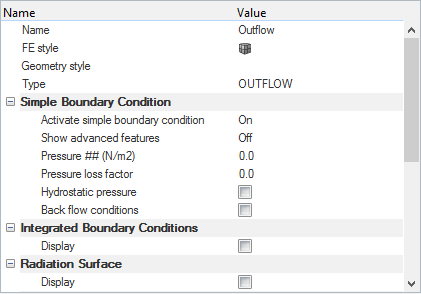
Figure 11. -
Click Wall. In the Entity Editor, verify that the Type is set to WALL.
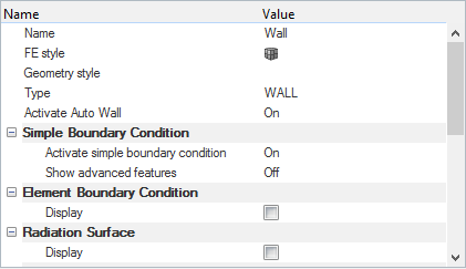
Figure 12. -
Click Slip_1. In the Entity Editor, change the Type to SLIP.
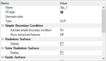
Figure 13.
Set the Nodal Initial Conditions
-
Under the Field tab, set the No. of Fields to 2 and
press Enter.
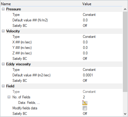
Figure 14.The Fields dialog opens. -
Set the fields as shown in the figure below.
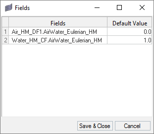
Figure 15.
Compute the Solution
In this step, you will launch AcuSolve directly from HyperMesh and compute the solution.
Run AcuSolve
-
Click
 on the ACU toolbar.
The Solver job Launcher dialog opens.
on the ACU toolbar.
The Solver job Launcher dialog opens. -
Leave the remaining options as
default and click Launch to start the solution
process.
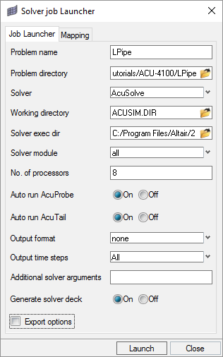
Figure 16.
Post-Process the Results with HyperView
Open HyperView and Load the Model and Results
-
In the Load model and results panel, click
 next
to Load model.
next
to Load model.
Create Contours for Volume Fraction of Water
-
In the Results Browser, set the Time to
1.5 sec.
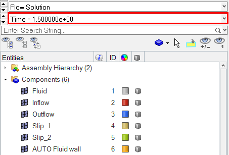
Figure 17. -
Click the Isolate shown icon
 and then click on the Fluid
component to turn off the display of all components except the Fluid
component.
and then click on the Fluid
component to turn off the display of all components except the Fluid
component.
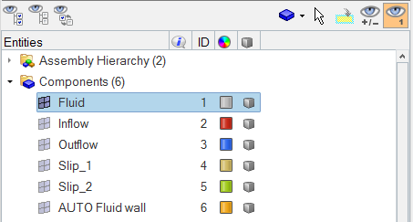
Figure 18. -
Orient the display to the xy-plane by clicking
 on the Standard Views toolbar.
-
Click
 on the Results toolbar to open the Contour panel.
-
In the panel area, under the Display tab, turn off
the Discrete color option.
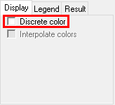
Figure 19. -
In the Edit Legend dialog, change the Numeric format to
Fixed. In the Values section, click on the Minimum
value in the legend and set it to 0.80. Similarly, set
the Maximum value to 1.0.
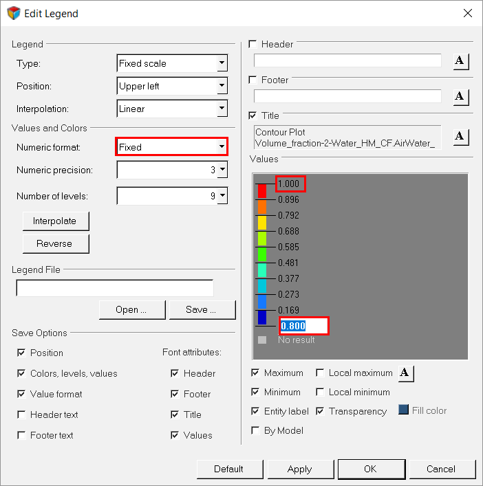
Figure 20. -
Verify that the contour plot looks like the figure below at frame 16.
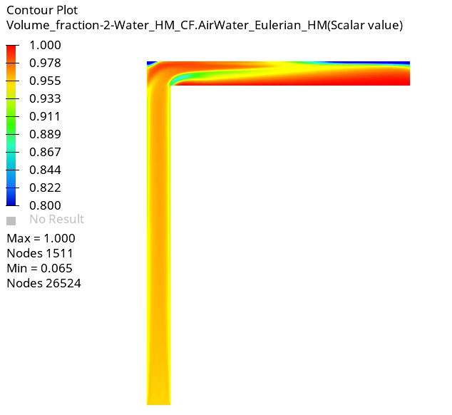
Figure 21.
Summary
In this tutorial, you worked through a basic workflow to set-up and solve a transient multiphase flow problem using the Algebraic Eulerian multiphase model using HyperWorks products, namely HyperMesh and AcuSolve. You started by importing the model in HyperMesh. Then, you defined the simulation parameters and launched AcuSolve directly from within HyperMesh. Upon completion of the solution by AcuSolve, you used HyperView to post-process the results and created a contour plot of the volume fraction.